Life Expectancy Analysis Report

Author

Mackenzie Hiddie, Adam Thomas, Huseen Munye, Yusuf Unsal, Austin Perkins, Justyn Kovalsk

Introduction

1.1 Data Understanding
1.2 Data Source
1.3 Initial Questions

Data Loading & Understanding

2.1 Importing Libraries
2.2 Loading and Understanding the Data
2.3 Categorizing the Datasets Attributes

Data Cleaning

3.1 Handling Null Values
3.2 Handling Outliers
- 3.2.2 Treating Outliers
- 3.2.3 Decision for Treating Outliers

Data Analysis

4.1 Plots
4.2 Variance Analysis
4.3 Covariance Analysis

Models

5.1 Multiple Regression of Life Expectancy
5.2 Neural Network of Life Expectancy
5.3 SVR Model for Life Expectancy
- 5.3.1 Conclusion of SVR Model
5.4 Random Forest
5.5 Which Variables Most Influence Life Expectancy
5.6 Comparing the Models
5.7 Predict Countries Economic Status from Life Expectancy
5.8 Deep Analysis
- 5.8.1 Deep Analysis Conclusion

Introduction

This dataset includes comprehensive information on 179 countries spanning from 2000 to 2015, covering aspects like life expectancy, health indicators, immunization rates, and economic and demographic data. Originally sourced from Kaggle, it underwent updates to rectify inaccuracies and missing values. Population, GDP, and life expectancy figures were updated from World Bank data, while data on vaccinations, alcohol consumption, BMI, HIV rates, mortality, and other health metrics were sourced from the World Health Organization. Additional information on schooling was gathered from the University of Oxford’s Our World in Data project. Missing values were addressed using strategies such as filling with the closest three-year average or the regional average. Countries with significant missing data were excluded, and the remaining countries were categorized based on their Gross National Income per capita into developed vs developing economies, following guidelines from organizations like the World Trade Organization and the UN.

1.1 Data Understanding

Columns in the dataset:

Country: List of the 179 countries
Region: 179 countries are distributed in 9 regions. E.g. Africa, Asia, Oceania, European Union, Rest of Europe and etc.
Year: Years observed from 2000 to 2015
Infant_deaths: Represents infant deaths per 1000 population
Under_five_deaths: Represents deaths of children under five years old per 1000 population
Adult_mortality: Represents deaths of adults per 1000 population
Alcohol_consumption: Represents alcohol consumption that is recorded in liters of pure alcohol per capita with 15+ years old
Hepatitis_B: Represents % of coverage of Hepatitis B (HepB3) immunization among 1-year-olds
Measles: Represents % of coverage of Measles containing vaccine first dose (MCV1) immunization among 1-year-olds
BMI: BMI is a measure of nutritional status in adults. It is defined as a person’s weight in kilograms divided by the square of that person’s height in meters (kg/m2)
Polio: Represents % of coverage of Polio (Pol3) immunization among 1-year-olds
Diphtheria: Represents % of coverage of Diphtheria tetanus toxoid and pertussis (DTP3) immunization among 1-year-olds
Incidents_HIV: Incidents of HIV per 1000 population aged 15-49
GDP_per_capita: GDP per capita in current USD
Population_mln: Total population in millions
Thinness_ten_nineteen_years: Prevalence of thinness among adolescents aged 10-19 years. BMI < -2 standard deviations below the median
Thinness_five_nine_years: Prevalence of thinness among children aged 5-9 years. BMI < -2 standard deviations below the median
Schooling: Average years that people aged 25+ spent in formal education
Economy_status_Developed: Developed country
Economy_status_Developing: Developing county
Life_expectancy: Average life expectancy of both genders in different years from 2010 to 2015

1.2 Data Source

Original dataset can be found here: https://www.kaggle.com/datasets/lashagoch/life-expectancy-who-updated

For ease of use we have re-uploaded the dataset to this Github repository created for this group project:

https://raw.githubusercontent.com/hmunye/life-expectancy-analysis/main/data/Life-Expectancy-Data-Updated.csv

1.3 Initial Questions

What are the predicting variables affecting life expectancy?
How does infant and adult mortality rates affect life expectancy?
Does life expectancy have a positive or negative correlation with
- BMI
- Diseases
- Alcohol Consumption
- Immunizations
What is the impact of schooling on the lifespan of humans?
- Can we predict lifespan based off of schooling?
Do densely populated countries tend to have lower life expectancy?
What is the impact of imunization coverage on life expectancy?
Will there be an increase in life expectancy in the next 10 years?
Will the rate of infant deaths go down over the next 5 years?
Is there a correlation between economic status and life expectancy?
- Can we predict countries economic status based off life expectancy?
Do certain regions have higher vaccination rates?

Data Loading & Understanding

2.1 Importing Libraries

Install these packages if not already installed on your machine:

options(repos = c(CRAN = "https://cloud.r-project.org"))

install.packages("tidyverse")

Installing package into '/opt/homebrew/lib/R/4.4/site-library'
(as 'lib' is unspecified)

install.packages("car")

Installing package into '/opt/homebrew/lib/R/4.4/site-library'
(as 'lib' is unspecified)

install.packages("caret")

Installing package into '/opt/homebrew/lib/R/4.4/site-library'
(as 'lib' is unspecified)

install.packages("neuralnet")

Installing package into '/opt/homebrew/lib/R/4.4/site-library'
(as 'lib' is unspecified)

install.packages("e1071")

Installing package into '/opt/homebrew/lib/R/4.4/site-library'
(as 'lib' is unspecified)

install.packages("randomForest")

Installing package into '/opt/homebrew/lib/R/4.4/site-library'
(as 'lib' is unspecified)

install.packages("caTools")

Installing package into '/opt/homebrew/lib/R/4.4/site-library'
(as 'lib' is unspecified)

install.packages("clusterGeneration")

Installing package into '/opt/homebrew/lib/R/4.4/site-library'
(as 'lib' is unspecified)

install.packages("pROC")

Installing package into '/opt/homebrew/lib/R/4.4/site-library'
(as 'lib' is unspecified)

install.packages("xgboost")

Installing package into '/opt/homebrew/lib/R/4.4/site-library'
(as 'lib' is unspecified)

Import the libraries:

library(tidyverse)

── Attaching core tidyverse packages ──────────────────────── tidyverse 2.0.0 ──
✔ dplyr     1.1.4     ✔ readr     2.1.5
✔ forcats   1.0.0     ✔ stringr   1.5.1
✔ ggplot2   3.5.1     ✔ tibble    3.2.1
✔ lubridate 1.9.3     ✔ tidyr     1.3.1
✔ purrr     1.0.2     
── Conflicts ────────────────────────────────────────── tidyverse_conflicts() ──
✖ dplyr::filter() masks stats::filter()
✖ dplyr::lag()    masks stats::lag()
ℹ Use the conflicted package (<http://conflicted.r-lib.org/>) to force all conflicts to become errors

library(caret)

Loading required package: lattice

Attaching package: 'caret'

The following object is masked from 'package:purrr':

    lift

library(car)

Loading required package: carData

Attaching package: 'car'

The following object is masked from 'package:dplyr':

    recode

The following object is masked from 'package:purrr':

    some

library(neuralnet)


Attaching package: 'neuralnet'

The following object is masked from 'package:dplyr':

    compute

library(e1071)
library(randomForest)

randomForest 4.7-1.1
Type rfNews() to see new features/changes/bug fixes.

Attaching package: 'randomForest'

The following object is masked from 'package:dplyr':

    combine

The following object is masked from 'package:ggplot2':

    margin

library(caTools)
library(parallel)
library(doParallel)

Loading required package: foreach

Attaching package: 'foreach'

The following objects are masked from 'package:purrr':

    accumulate, when

Loading required package: iterators

library(pROC)

Type 'citation("pROC")' for a citation.

Attaching package: 'pROC'

The following objects are masked from 'package:stats':

    cov, smooth, var

library(rpart)
library(rpart.plot)
library(xgboost)


Attaching package: 'xgboost'

The following object is masked from 'package:dplyr':

    slice

2.2 Loading and Understanding the Data

Load the dataset from the GitHub repository:

df <- read_csv("https://raw.githubusercontent.com/hmunye/life-expectancy-analysis/main/data/Life-Expectancy-Data-Updated.csv", show_col_types = FALSE)

Display the first 5 rows of the dataset:

head(df, 5)

# A tibble: 5 × 21
  Country Region          Year Infant_deaths Under_five_deaths Adult_mortality
  <chr>   <chr>          <dbl>         <dbl>             <dbl>           <dbl>
1 Turkiye Middle East     2015          11.1              13             106. 
2 Spain   European Union  2015           2.7               3.3            57.9
3 India   Asia            2007          51.5              67.9           201. 
4 Guyana  South America   2006          32.8              40.5           222. 
5 Israel  Middle East     2012           3.4               4.3            58.0
# ℹ 15 more variables: Alcohol_consumption <dbl>, Hepatitis_B <dbl>,
#   Measles <dbl>, BMI <dbl>, Polio <dbl>, Diphtheria <dbl>,
#   Incidents_HIV <dbl>, GDP_per_capita <dbl>, Population_mln <dbl>,
#   Thinness_ten_nineteen_years <dbl>, Thinness_five_nine_years <dbl>,
#   Schooling <dbl>, Economy_status_Developed <dbl>,
#   Economy_status_Developing <dbl>, Life_expectancy <dbl>

Shape of the data frame

# Get the number of rows
num_rows <- nrow(df)

# Get the number of columns
num_cols <- ncol(df)

# Print the results
cat("Number of rows:", num_rows, "\n")

Number of rows: 2864

cat("Number of columns:", num_cols, "\n")

Number of columns: 21

Summary of the Data Frame:

summary(df)

   Country             Region               Year      Infant_deaths   
 Length:2864        Length:2864        Min.   :2000   Min.   :  1.80  
 Class :character   Class :character   1st Qu.:2004   1st Qu.:  8.10  
 Mode  :character   Mode  :character   Median :2008   Median : 19.60  
                                       Mean   :2008   Mean   : 30.36  
                                       3rd Qu.:2011   3rd Qu.: 47.35  
                                       Max.   :2015   Max.   :138.10  
 Under_five_deaths Adult_mortality  Alcohol_consumption  Hepatitis_B   
 Min.   :  2.300   Min.   : 49.38   Min.   : 0.000      Min.   :12.00  
 1st Qu.:  9.675   1st Qu.:106.91   1st Qu.: 1.200      1st Qu.:78.00  
 Median : 23.100   Median :163.84   Median : 4.020      Median :89.00  
 Mean   : 42.938   Mean   :192.25   Mean   : 4.821      Mean   :84.29  
 3rd Qu.: 66.000   3rd Qu.:246.79   3rd Qu.: 7.777      3rd Qu.:96.00  
 Max.   :224.900   Max.   :719.36   Max.   :17.870      Max.   :99.00  
    Measles           BMI            Polio        Diphtheria   
 Min.   :10.00   Min.   :19.80   Min.   : 8.0   Min.   :16.00  
 1st Qu.:64.00   1st Qu.:23.20   1st Qu.:81.0   1st Qu.:81.00  
 Median :83.00   Median :25.50   Median :93.0   Median :93.00  
 Mean   :77.34   Mean   :25.03   Mean   :86.5   Mean   :86.27  
 3rd Qu.:93.00   3rd Qu.:26.40   3rd Qu.:97.0   3rd Qu.:97.00  
 Max.   :99.00   Max.   :32.10   Max.   :99.0   Max.   :99.00  
 Incidents_HIV     GDP_per_capita   Population_mln    
 Min.   : 0.0100   Min.   :   148   Min.   :   0.080  
 1st Qu.: 0.0800   1st Qu.:  1416   1st Qu.:   2.098  
 Median : 0.1500   Median :  4217   Median :   7.850  
 Mean   : 0.8943   Mean   : 11541   Mean   :  36.676  
 3rd Qu.: 0.4600   3rd Qu.: 12557   3rd Qu.:  23.688  
 Max.   :21.6800   Max.   :112418   Max.   :1379.860  
 Thinness_ten_nineteen_years Thinness_five_nine_years   Schooling     
 Min.   : 0.100              Min.   : 0.1             Min.   : 1.100  
 1st Qu.: 1.600              1st Qu.: 1.6             1st Qu.: 5.100  
 Median : 3.300              Median : 3.4             Median : 7.800  
 Mean   : 4.866              Mean   : 4.9             Mean   : 7.632  
 3rd Qu.: 7.200              3rd Qu.: 7.3             3rd Qu.:10.300  
 Max.   :27.700              Max.   :28.6             Max.   :14.100  
 Economy_status_Developed Economy_status_Developing Life_expectancy
 Min.   :0.0000           Min.   :0.0000            Min.   :39.40  
 1st Qu.:0.0000           1st Qu.:1.0000            1st Qu.:62.70  
 Median :0.0000           Median :1.0000            Median :71.40  
 Mean   :0.2067           Mean   :0.7933            Mean   :68.86  
 3rd Qu.:0.0000           3rd Qu.:1.0000            3rd Qu.:75.40  
 Max.   :1.0000           Max.   :1.0000            Max.   :83.80

2.3 Categorizing the Datasets Attributes

Nominal (Factors)
- Country
- Region
- Year
- Economy_status_Developed
- Economy_status_Developing
Numerical (Nominal):
- Infant_deaths
- Under_five_deaths
Numerical (Interval)
- BMI
Numerical (Ratio)
- Life_expectancy
- Adult_mortality
- Hepatitis_B
- Measles
- Polio
- Incidents_HIV
- GDP_per_capita
- Population_mln
- Thinness_five_nine_years
- Thinness_ten_nineteen_years
- Schooling

Creating a list of all nominal/factors

Regions

df |>
distinct(Region)

# A tibble: 9 × 1
  Region                       
  <chr>                        
1 Middle East                  
2 European Union               
3 Asia                         
4 South America                
5 Central America and Caribbean
6 Rest of Europe               
7 Africa                       
8 Oceania                      
9 North America

Country

df |>
distinct(Country)

# A tibble: 179 × 1
   Country           
   <chr>             
 1 Turkiye           
 2 Spain             
 3 India             
 4 Guyana            
 5 Israel            
 6 Costa Rica        
 7 Russian Federation
 8 Hungary           
 9 Jordan            
10 Moldova           
# ℹ 169 more rows

Year

df |>
distinct(Year)

# A tibble: 16 × 1
    Year
   <dbl>
 1  2015
 2  2007
 3  2006
 4  2012
 5  2000
 6  2001
 7  2008
 8  2011
 9  2002
10  2013
11  2005
12  2003
13  2004
14  2009
15  2010
16  2014

Economic Status:

df |>
distinct(Economy_status_Developed)

# A tibble: 2 × 1
  Economy_status_Developed
                     <dbl>
1                        0
2                        1

df |>
distinct(Economy_status_Developing)

# A tibble: 2 × 1
  Economy_status_Developing
                      <dbl>
1                         1
2                         0

For the purpose of analysis in R, it is good practice to change categorical variables into factors

df$Country <- factor(df$Country)
df$Region <- factor(df$Region)
df$Region <- factor(df$Region)
df$Year <- factor(df$Year)
df$Economy_status_Developed <- factor(df$Economy_status_Developed)
df$Economy_status_Developing <- factor(df$Economy_status_Developing)

glimpse(df)

Rows: 2,864
Columns: 21
$ Country                     <fct> "Turkiye", "Spain", "India", "Guyana", "Is…
$ Region                      <fct> Middle East, European Union, Asia, South A…
$ Year                        <fct> 2015, 2015, 2007, 2006, 2012, 2006, 2015, …
$ Infant_deaths               <dbl> 11.1, 2.7, 51.5, 32.8, 3.4, 9.8, 6.6, 8.7,…
$ Under_five_deaths           <dbl> 13.0, 3.3, 67.9, 40.5, 4.3, 11.2, 8.2, 10.…
$ Adult_mortality             <dbl> 105.8240, 57.9025, 201.0765, 222.1965, 57.…
$ Alcohol_consumption         <dbl> 1.32, 10.35, 1.57, 5.68, 2.89, 4.19, 8.06,…
$ Hepatitis_B                 <dbl> 97, 97, 60, 93, 97, 88, 97, 88, 97, 97, 96…
$ Measles                     <dbl> 65, 94, 35, 74, 89, 86, 97, 99, 87, 92, 70…
$ BMI                         <dbl> 27.8, 26.0, 21.2, 25.3, 27.0, 26.4, 26.2, …
$ Polio                       <dbl> 97, 97, 67, 92, 94, 89, 97, 99, 97, 96, 96…
$ Diphtheria                  <dbl> 97, 97, 64, 93, 94, 89, 97, 99, 99, 90, 95…
$ Incidents_HIV               <dbl> 0.08, 0.09, 0.13, 0.79, 0.08, 0.16, 0.08, …
$ GDP_per_capita              <dbl> 11006, 25742, 1076, 4146, 33995, 9110, 931…
$ Population_mln              <dbl> 78.53, 46.44, 1183.21, 0.75, 7.91, 4.35, 1…
$ Thinness_ten_nineteen_years <dbl> 4.9, 0.6, 27.1, 5.7, 1.2, 2.0, 2.3, 2.3, 4…
$ Thinness_five_nine_years    <dbl> 4.8, 0.5, 28.0, 5.5, 1.1, 1.9, 2.3, 2.3, 3…
$ Schooling                   <dbl> 7.8, 9.7, 5.0, 7.9, 12.8, 7.9, 12.0, 10.2,…
$ Economy_status_Developed    <fct> 0, 1, 0, 0, 1, 0, 0, 1, 0, 0, 0, 1, 0, 0, …
$ Economy_status_Developing   <fct> 1, 0, 1, 1, 0, 1, 1, 0, 1, 1, 1, 0, 1, 1, …
$ Life_expectancy             <dbl> 76.5, 82.8, 65.4, 67.0, 81.7, 78.2, 71.2, …

Data Cleaning

3.1 Handling Null Values

The original data set had several hundred missing values. While the data is publicly available as it is all published by the various nations of the world and the World Heath Organization, it is not feasible with our teams man hours to manually enter each missing value.

Number of Missing Values:

Life_expectancy: 10
Adult_mortality: 10
Infant_deaths: 0
Hepatitis_B: 553
Measles: 0
BMI: 34
Under_five_deaths: 0
Polio: 19
Incidents_HIV: 0
GDP_per_capita: 448
Population_mln: 652
Thinness_five_nine_years: 34
Schooling: 163

3.1.1 Treating Null Values

1) Delete the row: Possible for datasets with small number of NA’s, sadly that is not our dataset.

2) Replace the missing values with the average for that variable

3.1.2 Decision for Treating Null Values

When doing research on how to handle the missing values, Our group leader found a data set that has already “fixed” the missing values. This new data set first grouped each country into regions, from there the average value of each column was found by region. This is a very clean way to ensure that different regions do not effect each other, while still filling in the missing values.

3.1.3 Approach

The group moved forward with the “Fixed” dataset.

3.2 Handling Outliers

Function to find number of outliers and plot:

num_outliers <- function(data_set, column) {
  q1 <- quantile(column, 0.25)
  q3 <- quantile(column, 0.75)
  iqr <- q3 -q1
  
  upper_bound <- q3 + 1.5 * iqr
  lower_bound <- q1 - 1.5 * iqr
  
  outliers <- column[column < lower_bound | column > upper_bound]
  
  plot <- ggplot(data_set) + geom_boxplot(aes(x = "", y = column))
  
  print(plot)
  
  return(length(outliers))
}

Number of Outliers:

Life_expectancy:

num_outliers(df, df$Life_expectancy)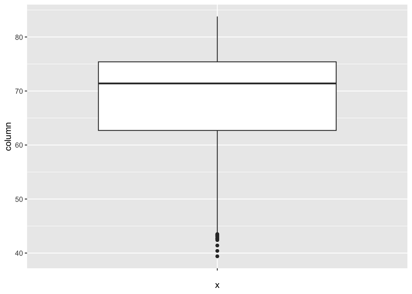

[1] 19

Adult_mortality:

num_outliers(df, df$Adult_mortality)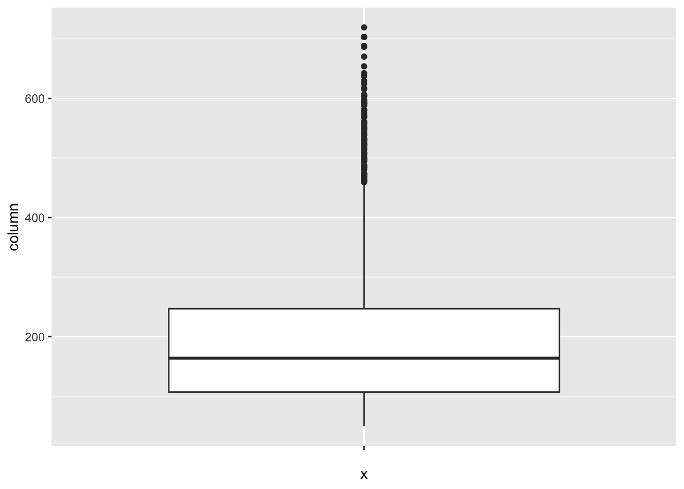

[1] 112

Alcohol_consumption:

num_outliers(df, df$Alcohol_consumption)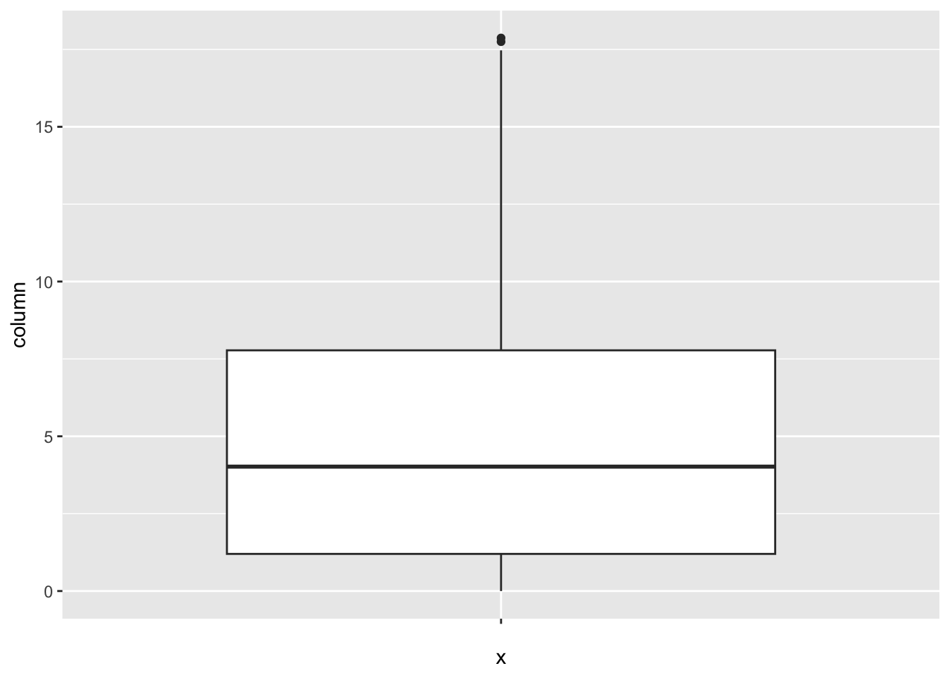

[1] 2

Hepatitis_B:

num_outliers(df, df$Hepatitis_B)

[1] 164

Measles:

num_outliers(df, df$Measles)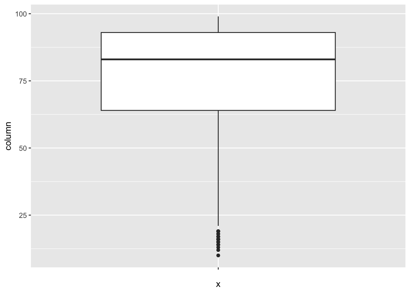

[1] 35

Polio:

num_outliers(df, df$Polio)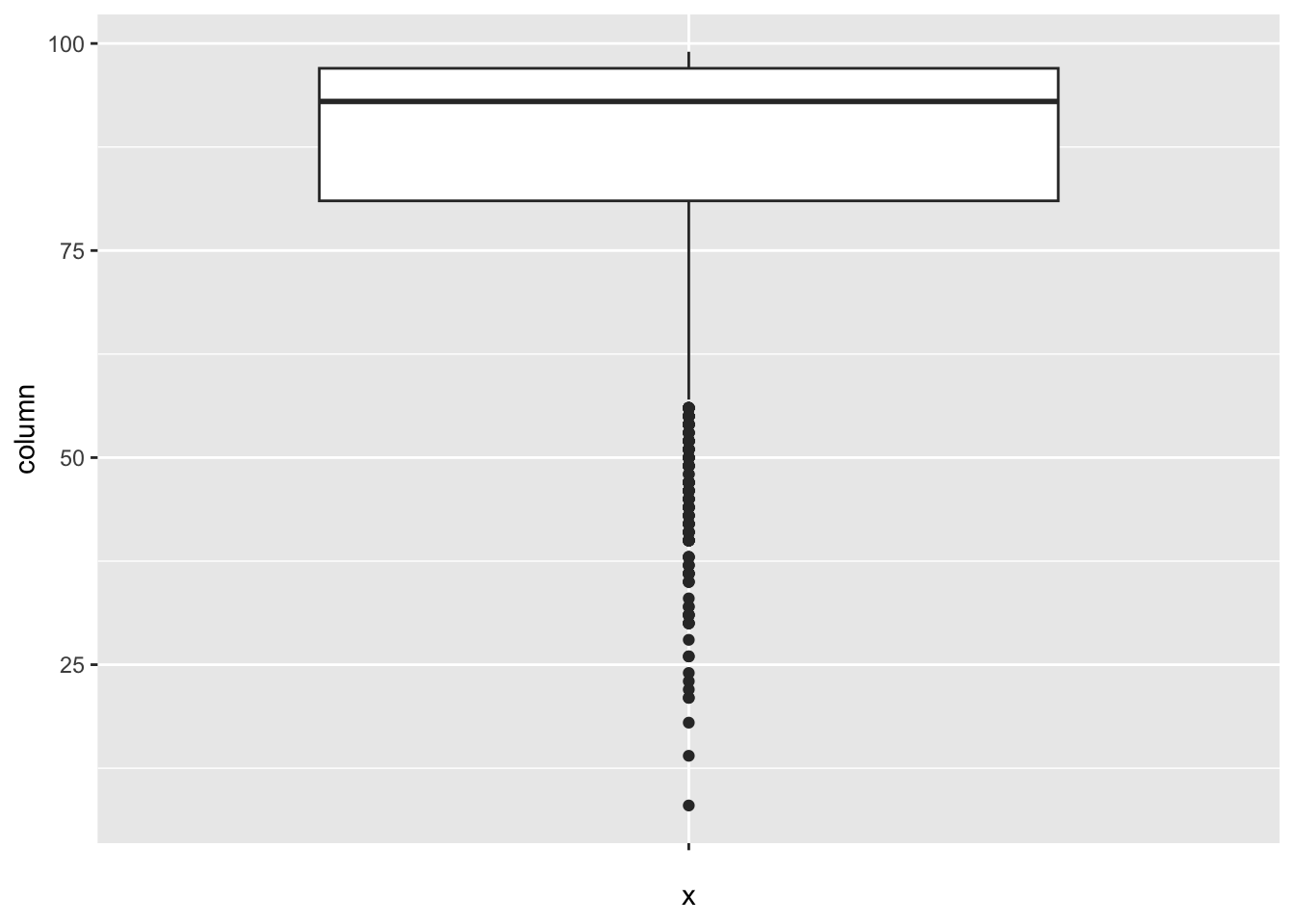

[1] 190

Diphtheria:

num_outliers(df, df$Diphtheria)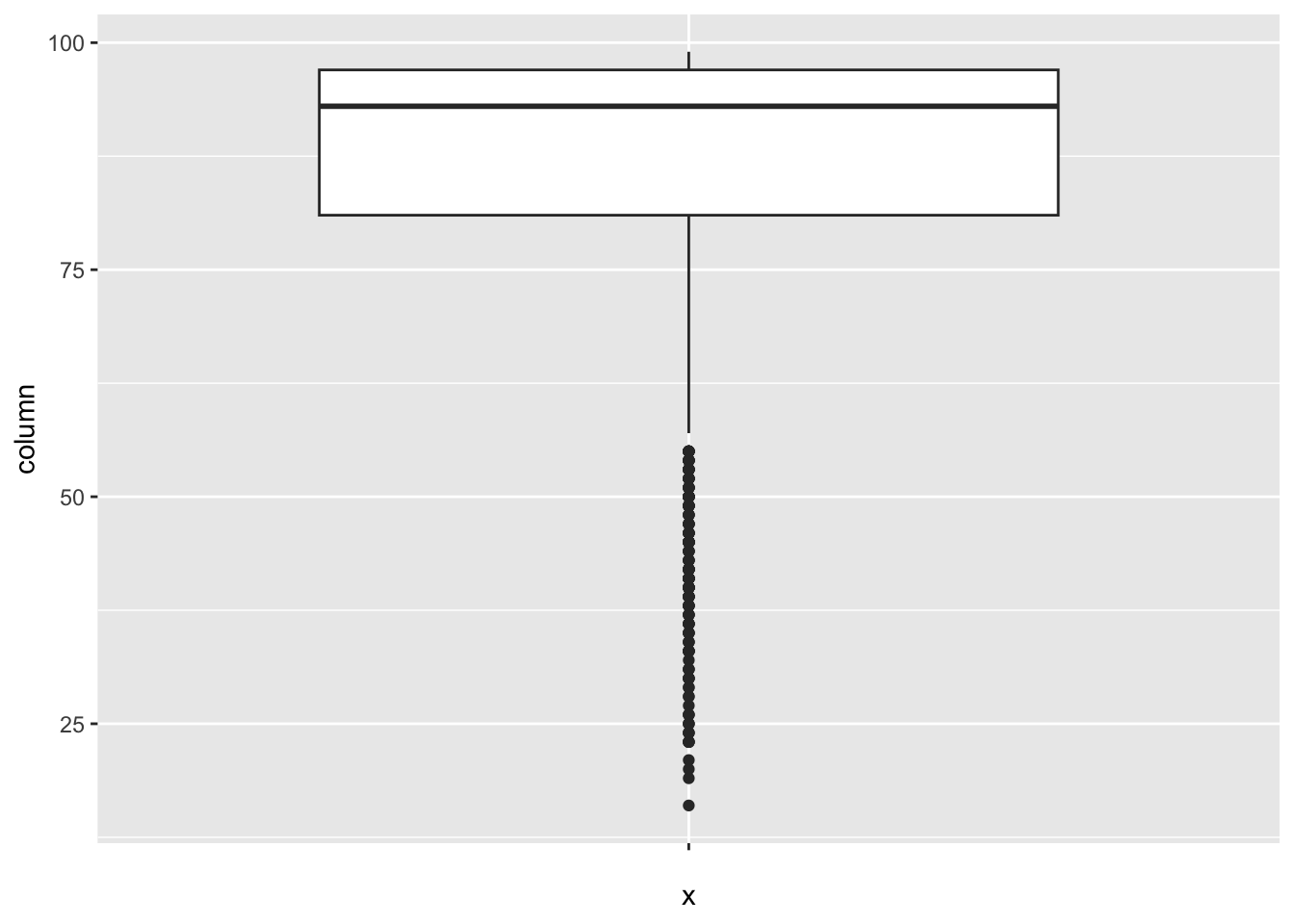

[1] 187

Incidents_HIV:

num_outliers(df, df$Incidents_HIV)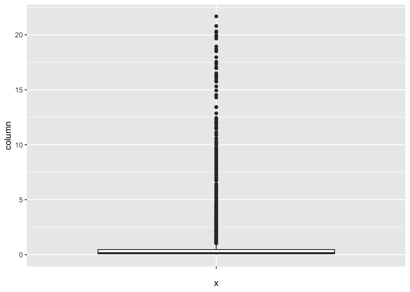

[1] 461

GDP_per_capita:

num_outliers(df, df$GDP_per_capita)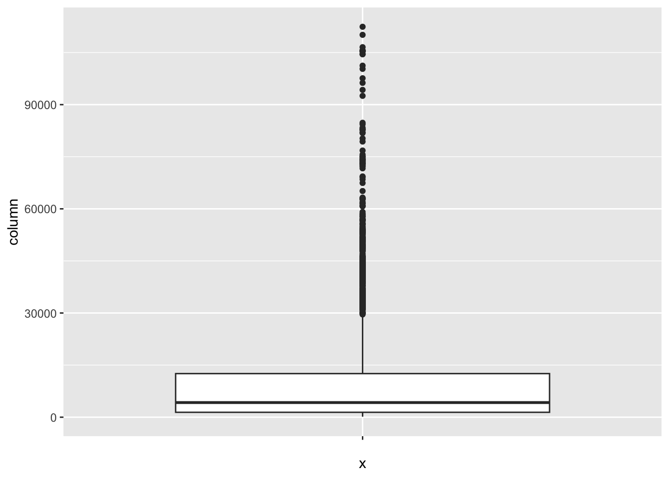

[1] 425

Population_mln:

num_outliers(df, df$Population_mln)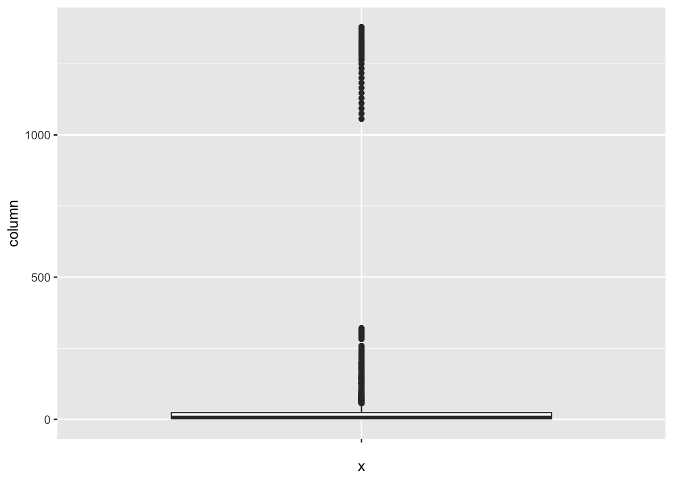

[1] 362

Thinness_five_nine_years:

num_outliers(df, df$Thinness_five_nine_years)

[1] 95

Thinness_ten_nineteen_years:

num_outliers(df, df$Thinness_ten_nineteen_years)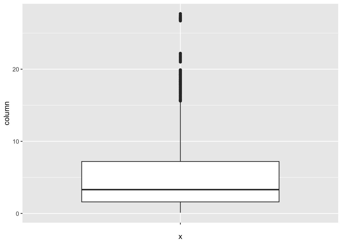

[1] 89

Schooling:

num_outliers(df, df$Schooling)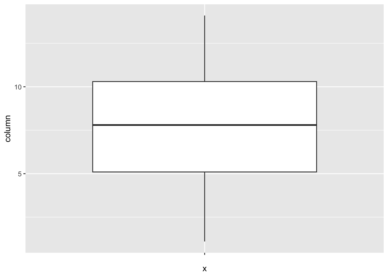

[1] 0

BMI:

num_outliers(df, df$BMI)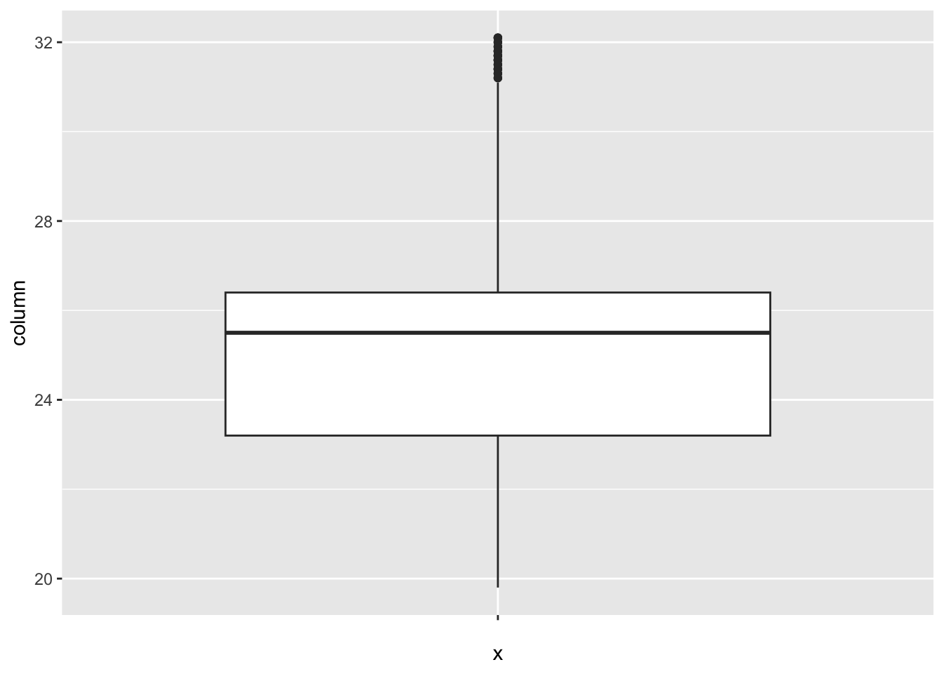

[1] 25

Infant_deaths:

num_outliers(df, df$Infant_deaths)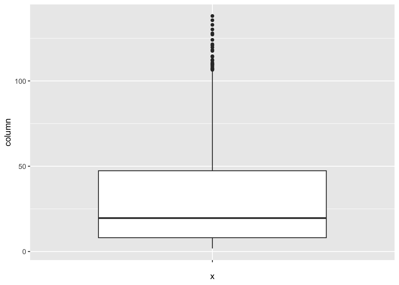

[1] 29

Under_five_deaths:

num_outliers(df, df$Under_five_deaths)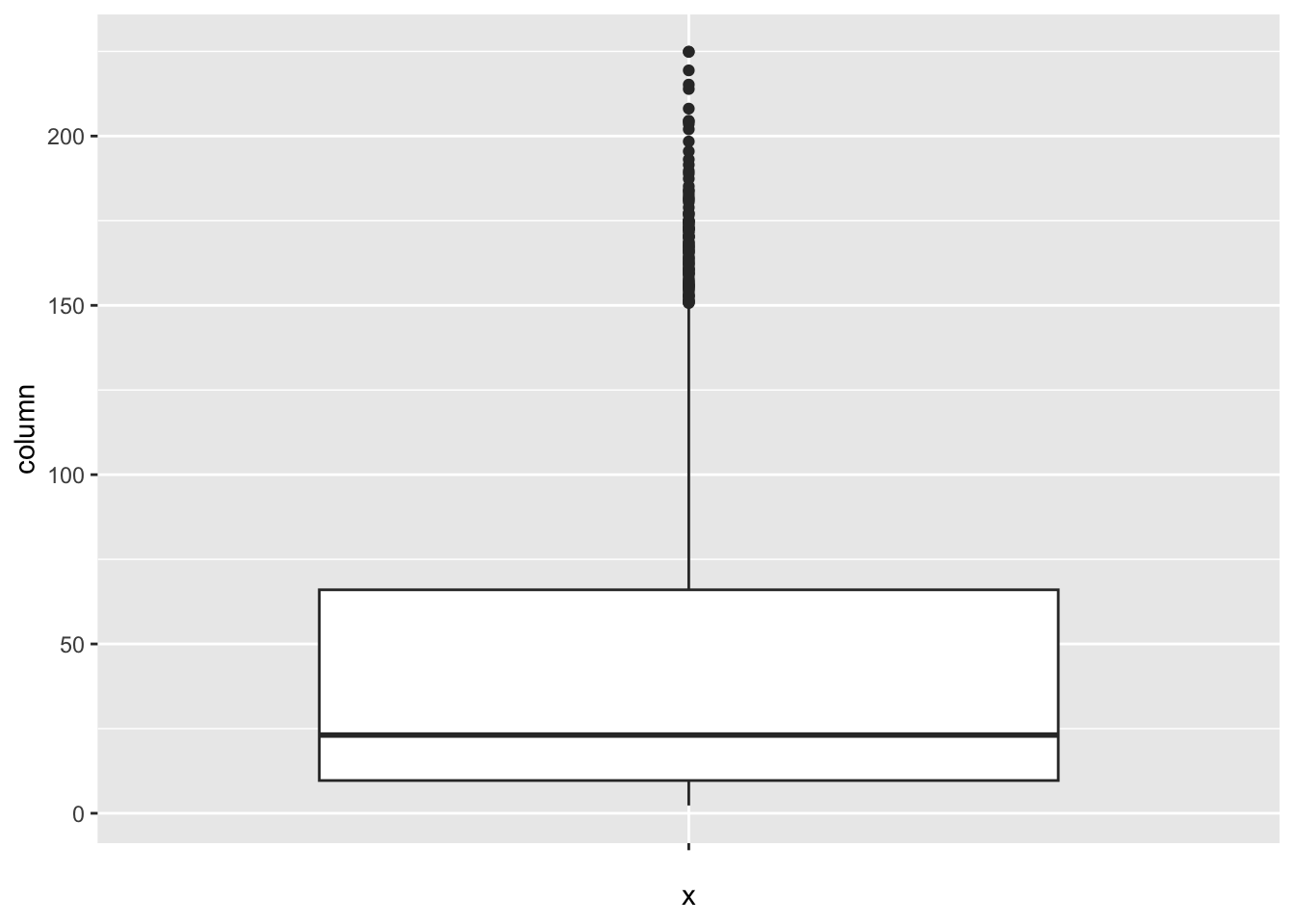

[1] 102

3.2.1 Explanation & Insights:

The variation in outlier counts between our analytical methods (IQR Method, identify_outliers function) and box plot visualization likely comes from differing definitions of outliers. While the analytical methods stick to strict statistical criteria, box plots visually show points beyond the data’s central range, potentially capturing more extreme values.

ggplot(df, aes(x = Region, y = Infant_deaths)) + geom_boxplot() + ggtitle("Comparison of Infant Deaths Incidence by Region")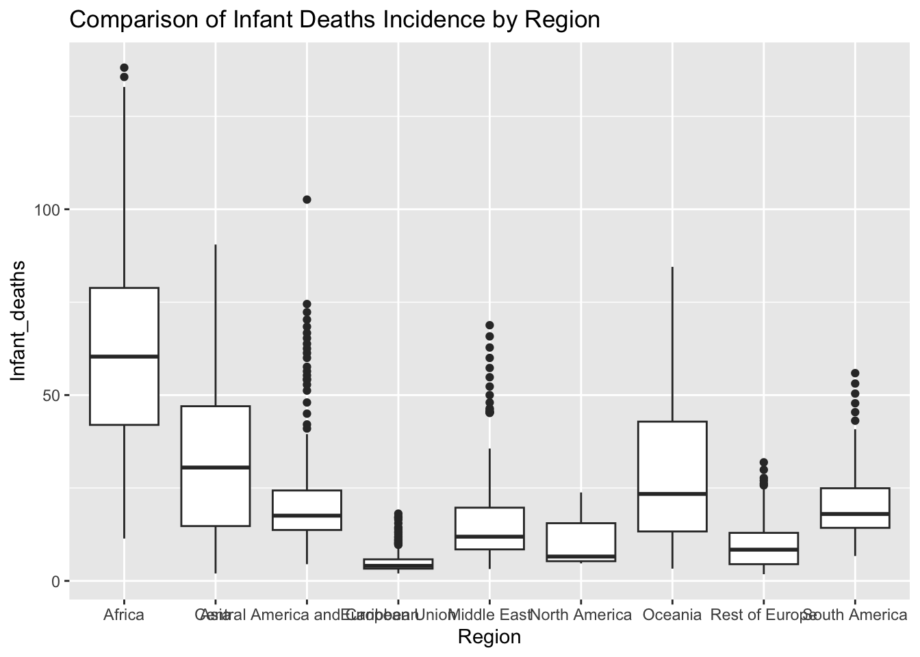

The “Infant_deaths” column represents the number of infant deaths per 1000 population. The IQR method identifies 29 outliers. The regions with outliers include Africa, Central America and Caribbean, European Union, Middle East, Rest of Europe, and South America. Outliers in infant deaths may indicate regions with unusually high infant mortality rates, potentially reflecting poor healthcare access and quality.

ggplot(df, aes(x = Region, y = Under_five_deaths )) + geom_boxplot() + ggtitle("Comparison of Under Five Deaths:  by Region")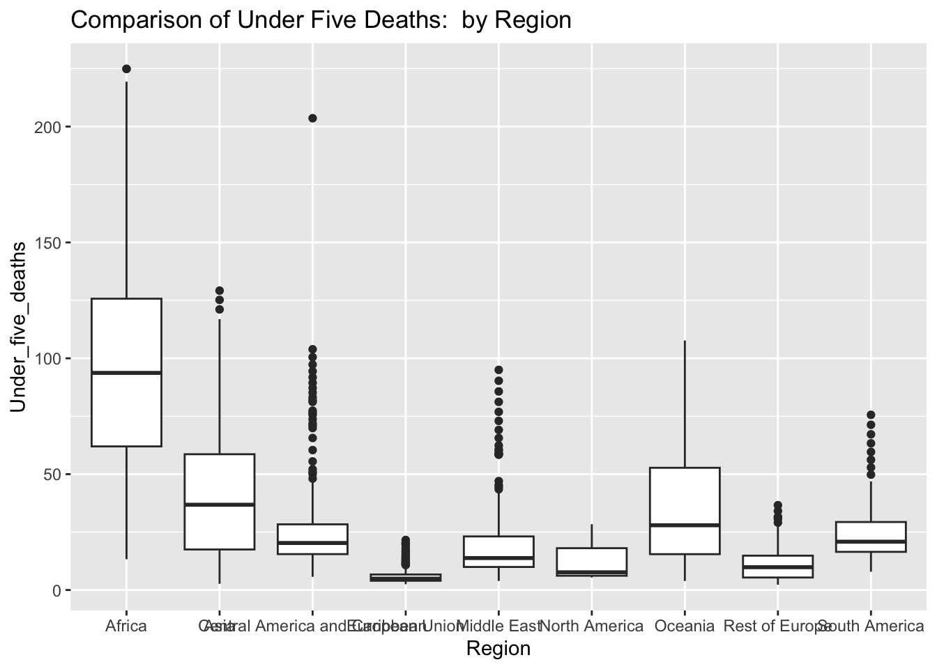

The “Under_five_deaths” column represents deaths of children under five years old per 1000 population. The IQR method identifies 102 outliers. The regions with outliers include Africa, Asia, Central America and Caribbean, European Union, Middle East, Rest of Europe, and South America. High rates of under-five deaths may indicate challenges related to healthcare access, quality, and availability of essential services such as maternal and child healthcare and vaccinations.

ggplot(df, aes(x = Region, y = Adult_mortality)) + geom_boxplot() + ggtitle("Comparison of Adult M         ortality by Region")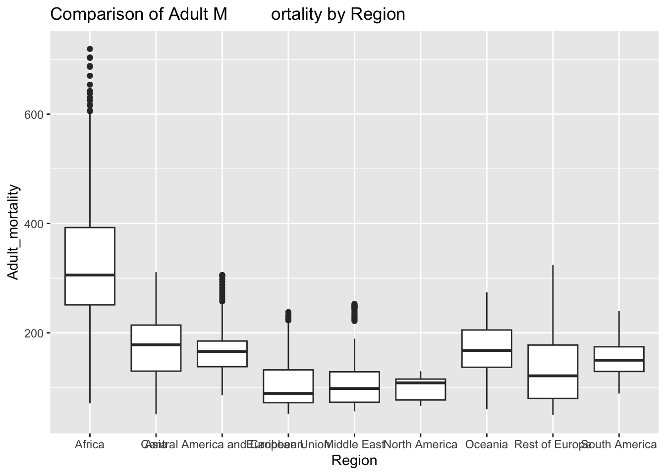

The “Adult_mortality” column represents the probability of dying between 15 and 60 per 1000 population. The IQR method identifies 112 outliers. The only region with outliers is Africa. High rates of adult mortality may indicate challenges related to healthcare access, quality, and availability of essential services such as vaccinations.

ggplot(df, aes(x = Region, y = Alcohol_consumption)) + geom_boxplot() + ggtitle("Comparison of Alcohol Consumption by Region")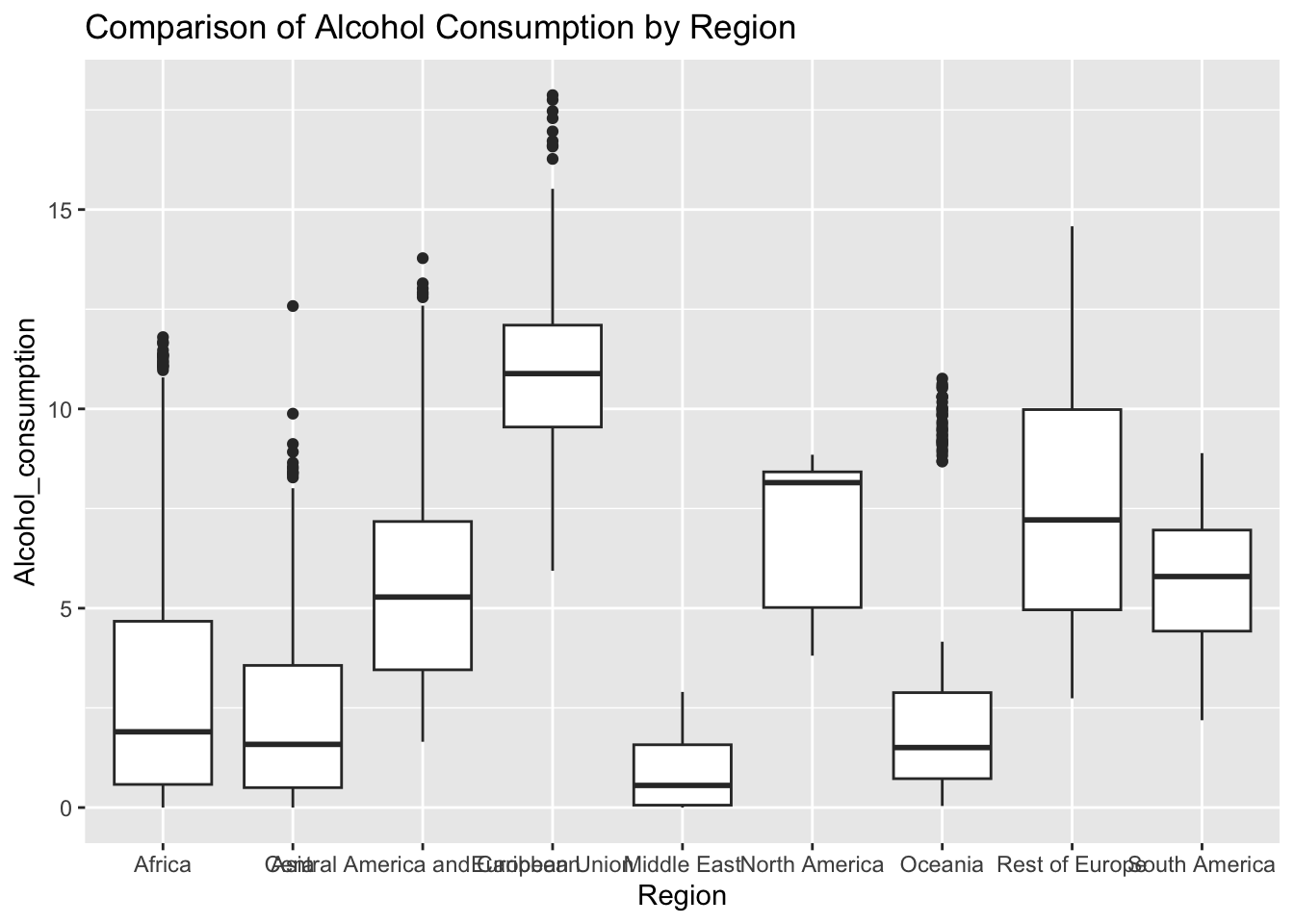

The “Alcohol_consumption” column represents alcohol consumption per capita by liter. The IQR method identifies 2 outliers.

ggplot(df, aes(x = Region, y = Hepatitis_B)) + geom_boxplot() + ggtitle("Comparison of Hepatitis B by Region")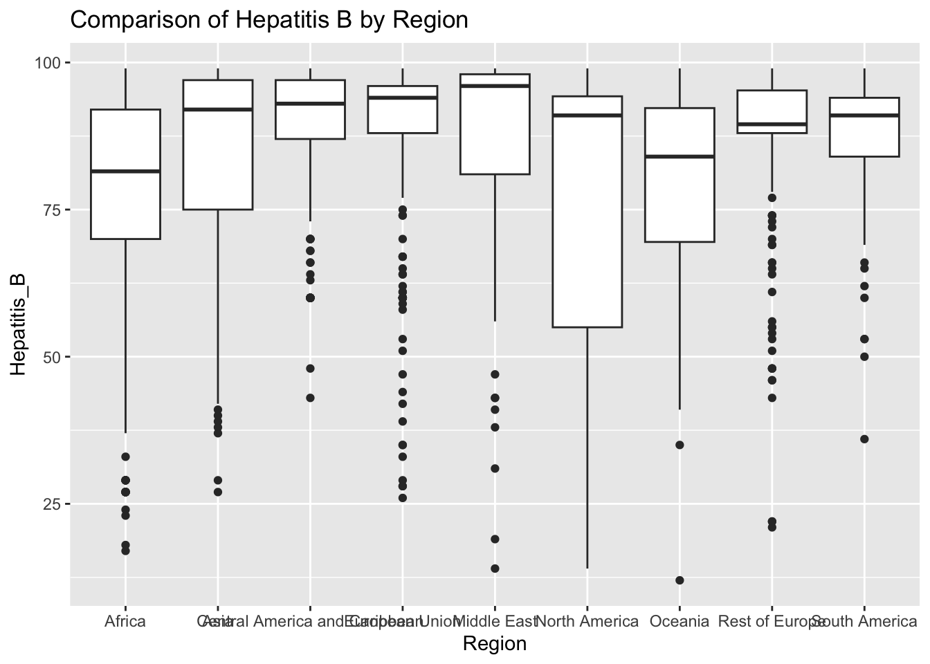

The “Hepatitis_B” column represents Hepatitis B immunization coverage in 1-year olds. The IQR method identifies 164 outliers.

ggplot(df, aes(x = Region, y = Measles)) + geom_boxplot() + ggtitle("Comparison of Measles by Region")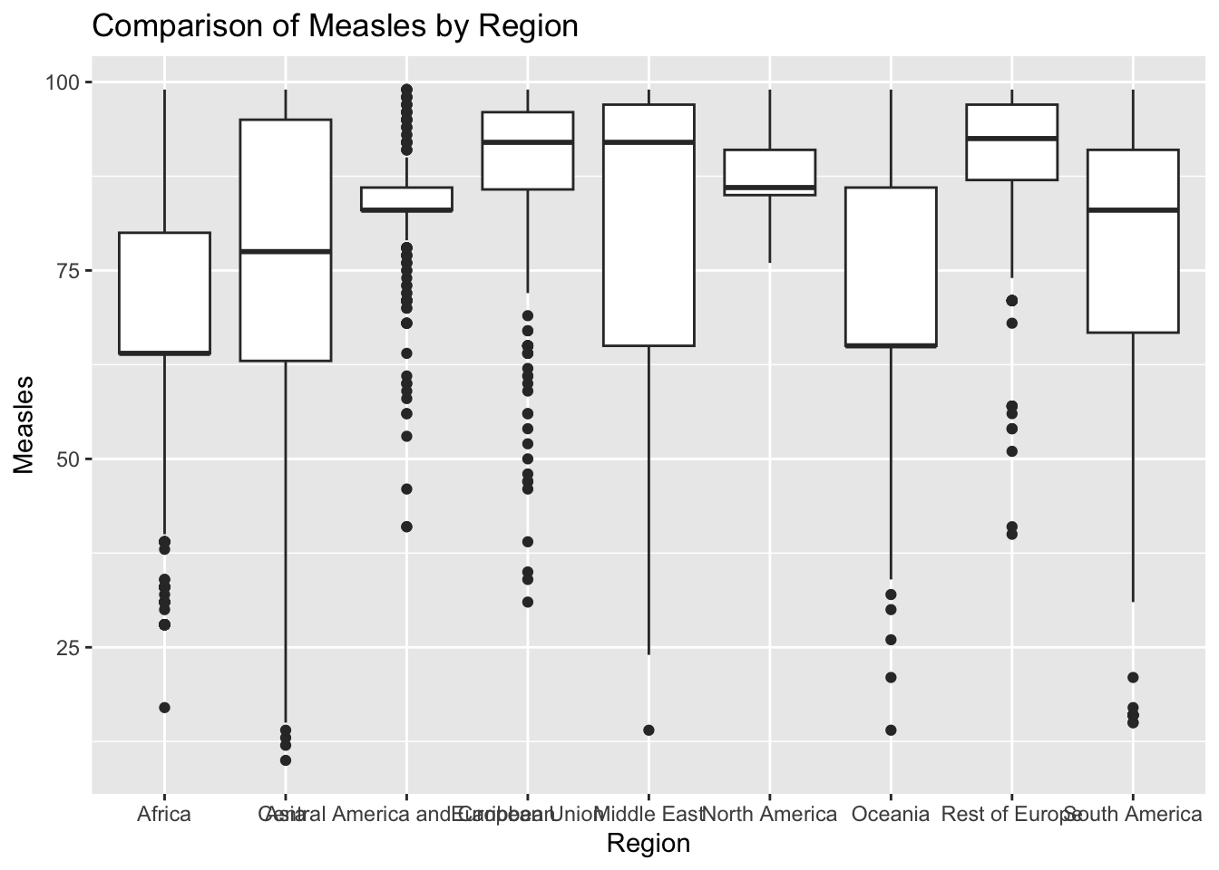

The “Measles” column represents number of measles cases reported per 1000 population. The IQR method identifies 35 outliers. The regions with outliers include Indonesia(Asia), Philippines(Asia), Afghanistan(Asia), and Suriname(South America). High rates of measles may indicate challenges related to healthcare access.

ggplot(df, aes(x = Region, y = BMI)) + geom_boxplot() + ggtitle("Comparison of BMI by Region")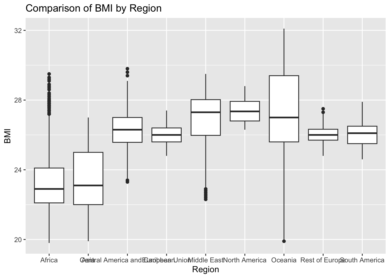

The “BMI” column represents the body mass index of the entire population. The IQR method identifies 25 outliers. The regions with outliers are Samoa and Tonga. Higher BMI may indicate genetic predispositions and fattier diets.

ggplot(df, aes(x = Region, y = Polio)) + geom_boxplot() + ggtitle("Comparison of Polio by Region")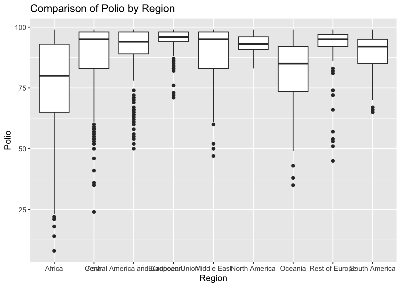

The “Polio” column represents the polio immunization records among 1-year olds. The IQR method identifies 190 outliers. The regions with outliers include Africa and Oceania. Lower polio vaccination rates may indicate challenges related to healthcare access.

ggplot(df, aes(x = Region, y = Diphtheria)) + geom_boxplot() + ggtitle("Comparison of Diphtheria by Region")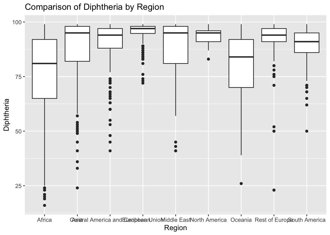

The “Diphtheria” column represents the TDP immunization records among 1-year olds. The IQR method identifies 187 outliers. The regions with outliers include Africa and Asia. Lower diphtheria vaccination rates may indicate challenges related to healthcare access.

ggplot(df, aes(x = Region, y = Incidents_HIV)) + geom_boxplot() + ggtitle("Comparison of Incidents HIV by Region")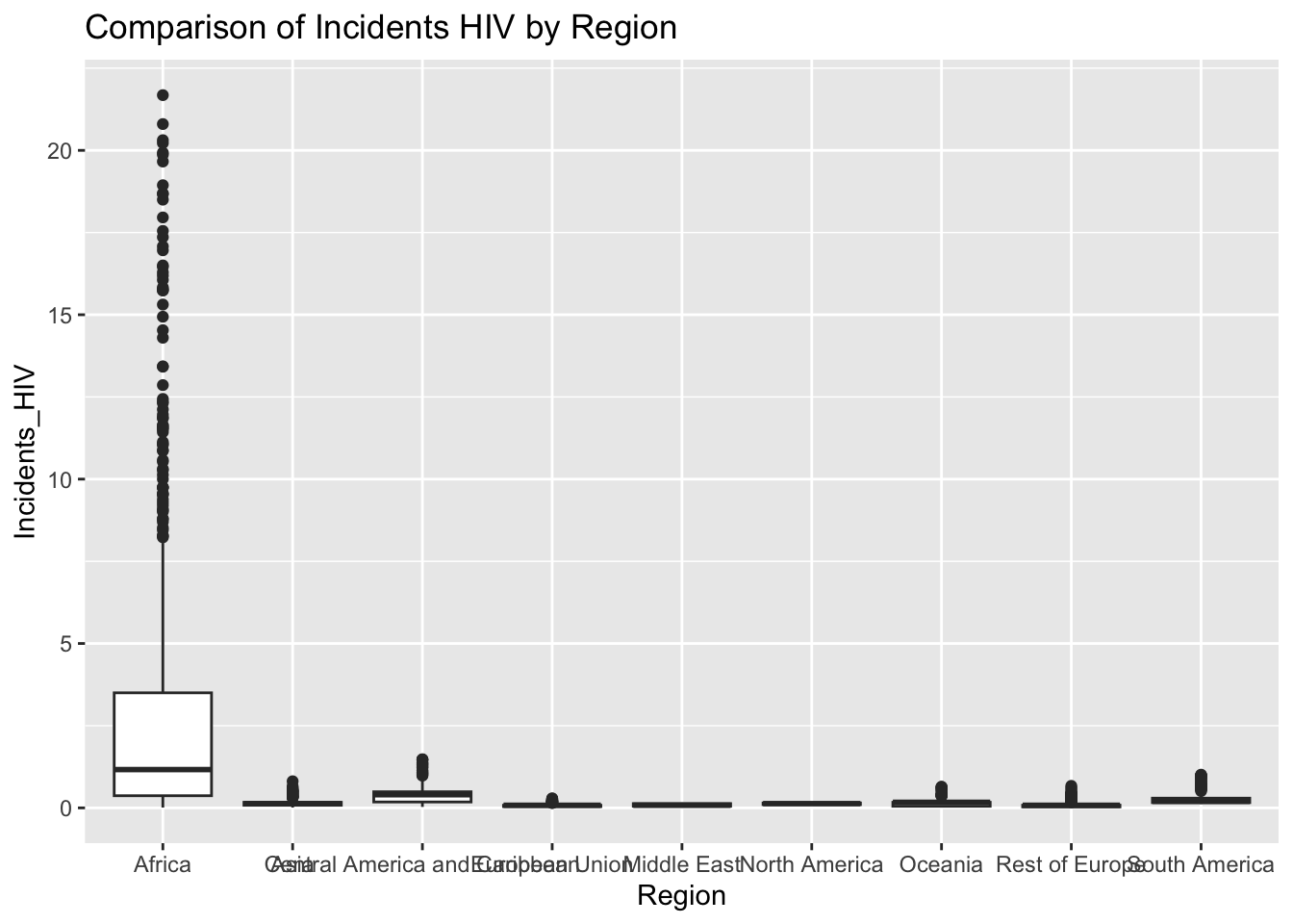

The “Incidents_HIV” column represents the deaths per 1000 live births due to HIV/AIDS. The IQR method identifies 461 outliers. The region with outliers is Africa. Higher HIV rates may indicate challenges related to healthcare access.

ggplot(df, aes(x = Region, y = GDP_per_capita)) + geom_boxplot() + ggtitle("Comparison of GDP Per Capita by Region")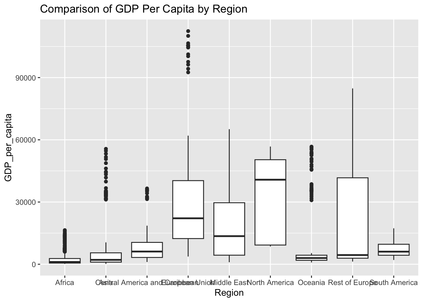

The “GDP_per_capita’ column represents the gross domestic product per capita. The IQR method identifies 425 outliers. The regions with outliers includes France and Austria. Higher GDP may indicate a more developed economy.

ggplot(df, aes(x = Region, y = Population_mln)) + geom_boxplot() + ggtitle("Comparison of Population by Region")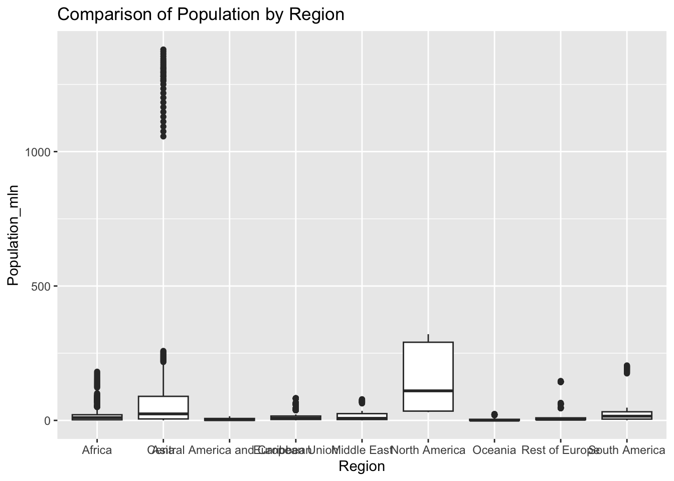

The “Population_mln” column represents the total population in millions. The IQR method identifies 362 outliers. The regions with outliers include India, China, and the United States.

ggplot(df, aes(x = Region, y = Thinness_ten_nineteen_years)) + geom_boxplot() + ggtitle("Comparison of Thinness Ten to Nineteen Years by Region")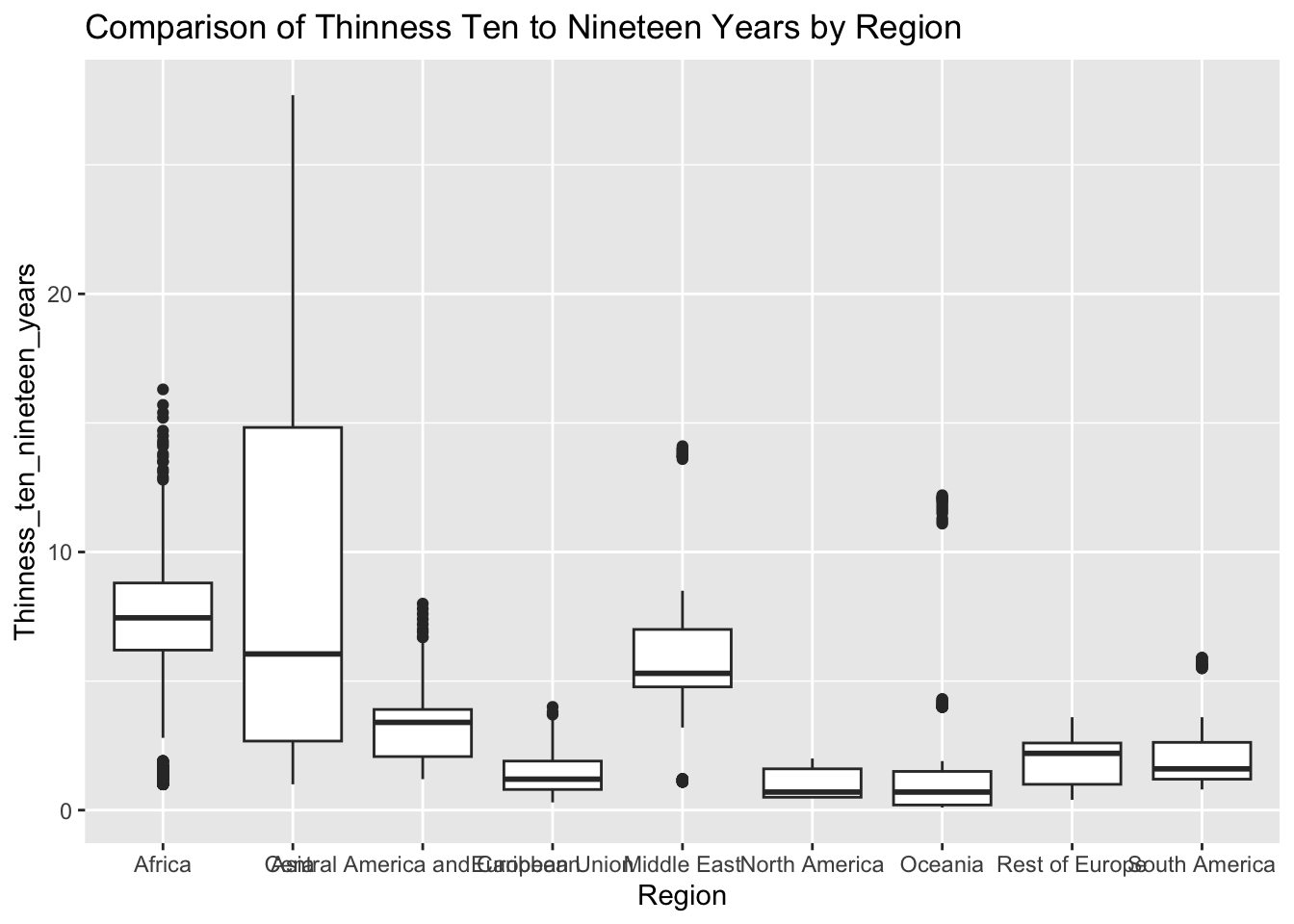

The “Thinness_ten_nineteen_years” column represents the prevalence of thinness among 10 to 19 year olds. The IQR method identifies 89 outliers. The regions with outliers include Asia and Africa. Higher rates of thinness may indicate challenges related to healthcare access, diet, and cultural values.

ggplot(df, aes(x = Region, y = Thinness_five_nine_years)) + geom_boxplot() + ggtitle("Comparison of Thinness Five to Nine Years by Region")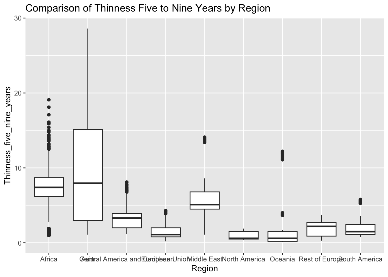

The “Thinness_five_nine_years” column represents the prevalence of thinness among 5 to 9 year olds. The IQR method identifies 95 outliers. The regions with outliers include Asia and Africa. Higher rates of thinness may indicate challenges related to healthcare access, diet, and cultural values.

ggplot(df, aes(x = Region, y = Schooling)) + geom_boxplot() + ggtitle("Comparison of Schooling by Region")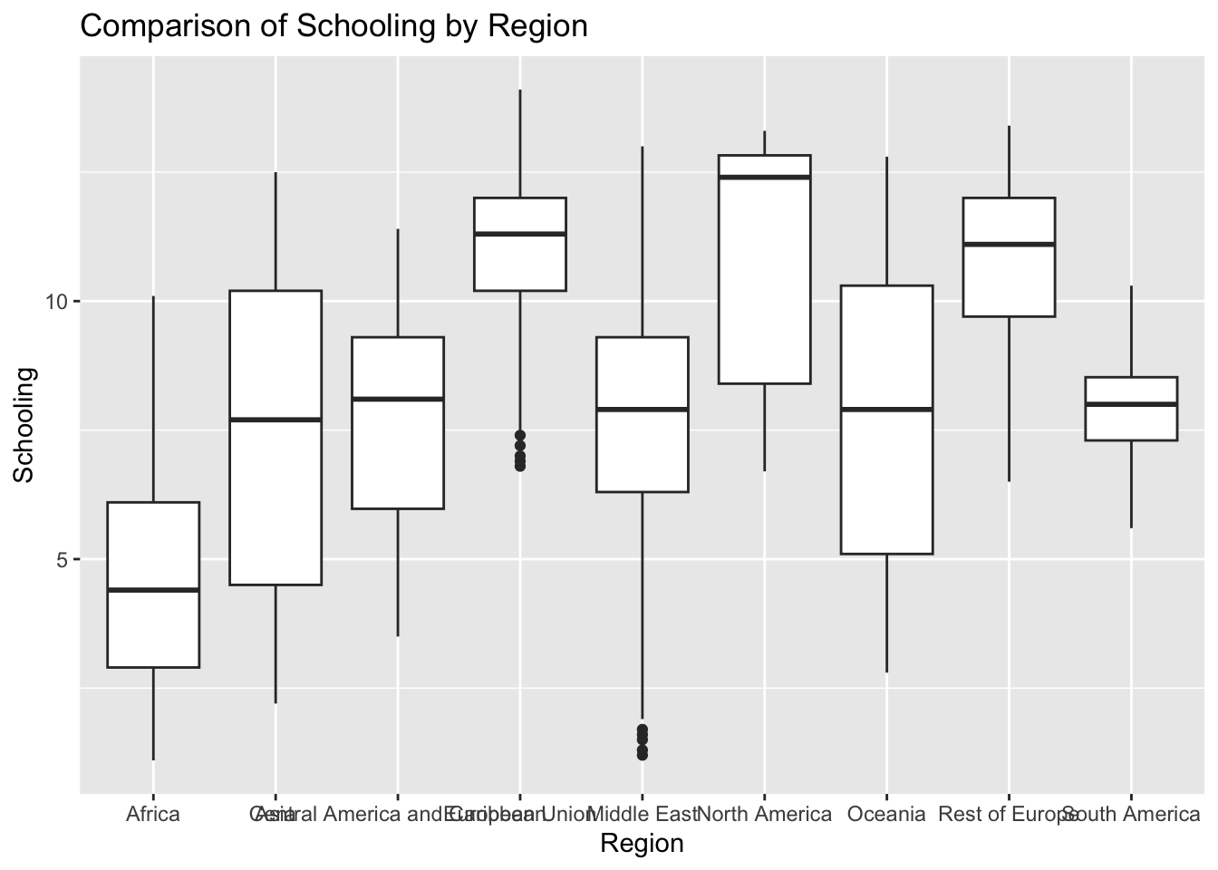

There are no outliers.

ggplot(df, aes(x = Region, y = Life_expectancy)) + geom_boxplot() + ggtitle("Comparison of Life Expectancy by Region")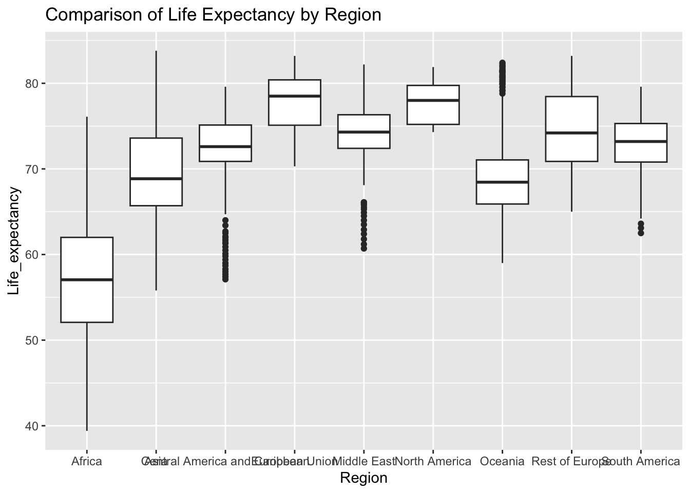

The “Life_expectancy” represents the average life expectancy in age. The IQR method identifies 19 outliers. The region with outliers include Africa. Lower life expectancy rates may indicate challenges related to healthcare access.

3.2.2 Treating Outliers

1) Trimming: Remove outliers from the dataset. This approach can be appropriate if the outliers are deemed to be data entry errors or highly improbable values. Due to the high number of outliers in the dataset, this is not a viable option.

2) Winsorization: Replace outliers with values at a specified percentile (e.g., replacing values above the 95th percentile with the 95th percentile value, replacing values below the 5th percentile with the 5th percentile value).

3.2.3 Decision for Treating Outliers

After doing research on how to identify and treat outliers in R, and reviewing the outliers present in our data, we have chosen to leave the outliers as is. None of them appear erroneous and as such provide valid data for training the models

Data Analysis

4.1 Plots

covariance_plot <- function(y_val, x_val, data_frame, std_data_frame) {
  ggplot(data = data_frame, aes_string(y = y_val, x = x_val, color = "Region")) +
    geom_point() +
    geom_text(aes(label = paste("Covariance:", round(cov(std_data_frame[[y_val]], std_data_frame[[x_val]]), 2))),
            x = Inf, y = Inf, hjust = 1, vjust = 1, color = "black")
}

4.2 Variance Analysis

Life Expectancy

df |>
ggplot() +
    geom_boxplot(aes(x=0, y=df$Life_expectancy))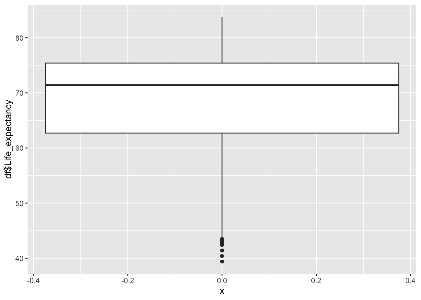

df |>
ggplot() +
    geom_histogram(aes(x=df$Life_expectancy), bins = 30)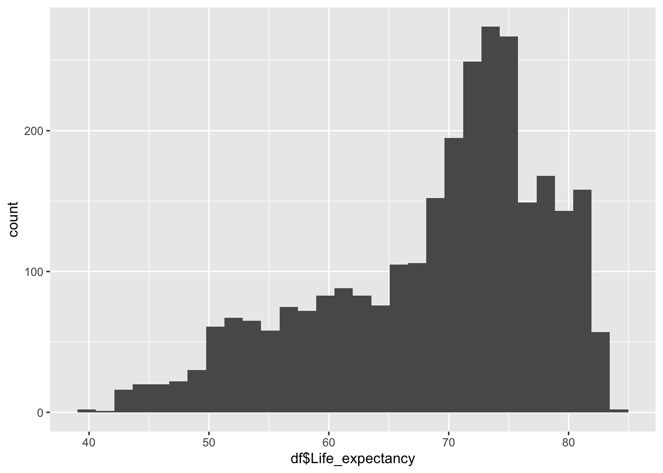

ggplot(df, aes(x=Life_expectancy, fill=Region)) +
    geom_histogram(bins=30, alpha=0.6, position="identity") +
    labs(title="Histogram of Life expectancy by Region",
         x="Life expectancy",
         y="Count") +
    theme_minimal()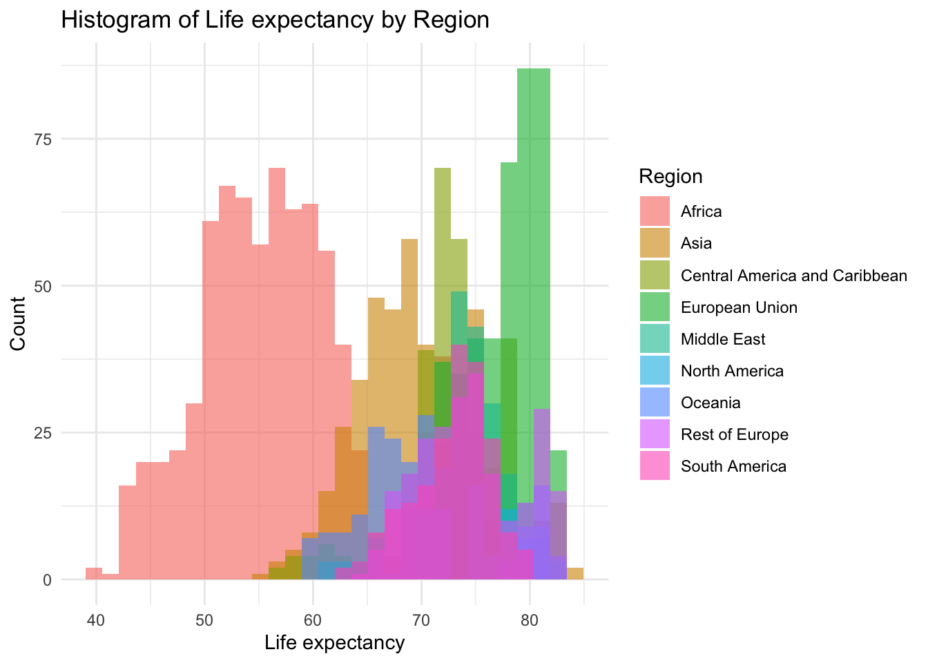

summary(df$Life_expectancy)

   Min. 1st Qu.  Median    Mean 3rd Qu.    Max. 
  39.40   62.70   71.40   68.86   75.40   83.80

Inference:

Life Expectancy represents the average years lived in the given country

Life Expectancy is not evenly distributed,

Life Expectancy peaks ~71

The minimum is 39.40, the max is 83.8

We can see that the various regions are clustered

Infant Deaths

df |>
ggplot() +
    geom_boxplot(aes(x=0, y=df$Infant_deaths))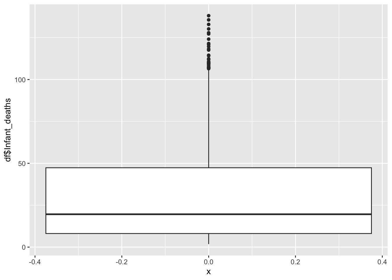

df |>
ggplot() +
    geom_histogram(aes(x=df$Infant_deaths), bins = 30)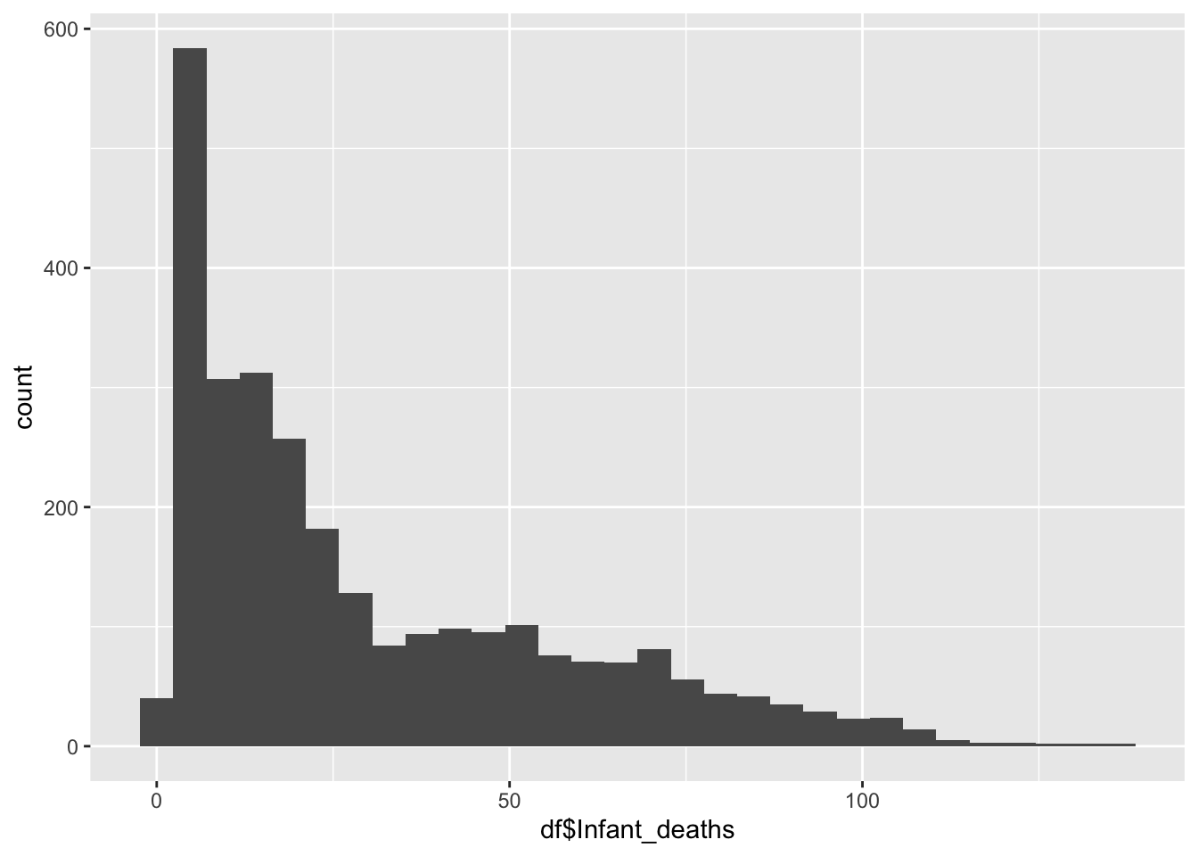

ggplot(df, aes(x=Life_expectancy, fill=Region)) +
    geom_histogram(bins=30, alpha=0.6, position="identity") +
    labs(title="Histogram of Infant_deaths by Region",
         x="Infant deaths",
         y="Count") +
    theme_minimal()

summary(df$Infant_deaths)

   Min. 1st Qu.  Median    Mean 3rd Qu.    Max. 
   1.80    8.10   19.60   30.36   47.35  138.10

Inference:

It represents the Infant Deaths in the given country

Life Expectancy is not evenly distributed,

Life Expectancy peaks ~20

The minimum is 1.80, the max is 138.10

Under_five_deaths

df |>
ggplot() +
    geom_boxplot(aes(x=0, y=df$Under_five_deaths))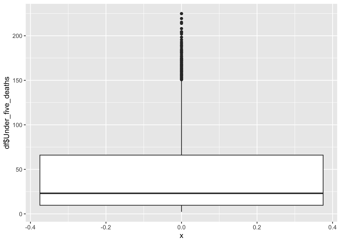

df |>
ggplot() +
    geom_histogram(aes(x=df$Under_five_deaths), bins = 30)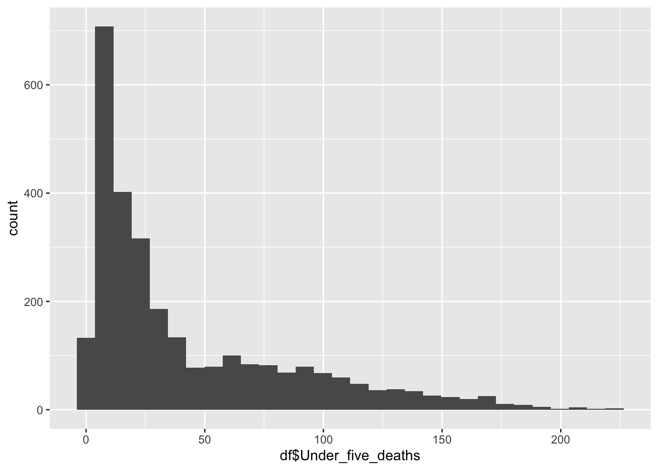

ggplot(df, aes(x=Under_five_deaths, fill=Region)) +
    geom_histogram(bins=30, alpha=0.6, position="identity") +
    labs(title="Histogram of Under_five_deaths by Region",
         x="Under_five_deaths",
         y="Count") +
    theme_minimal()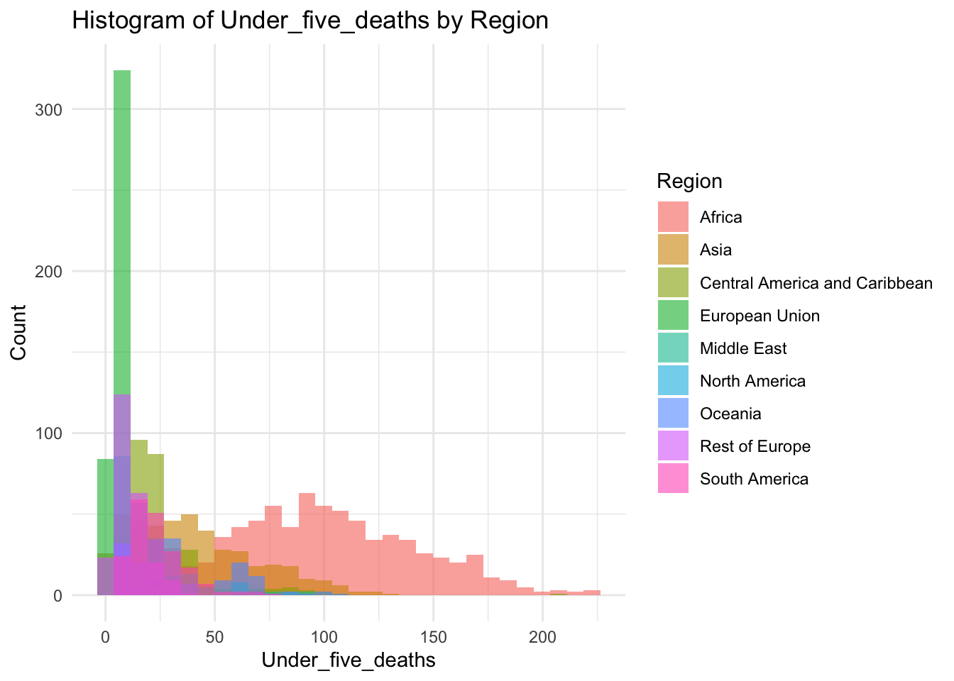

summary(df$Under_five_deaths)

   Min. 1st Qu.  Median    Mean 3rd Qu.    Max. 
  2.300   9.675  23.100  42.938  66.000 224.900

Inference:

Life Expectancy represents the average deaths under five (age) in the given country

Life Expectancy is not evenly distributed,

Life Expectancy peaks ~23

The minimum is 2.30, the max is 224.90

Adult_mortality

df |>
ggplot() +
    geom_boxplot(aes(x=0, y=df$Adult_mortality))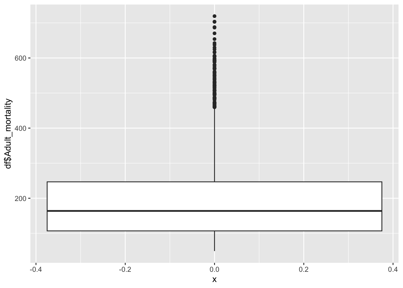

df |>
ggplot() +
    geom_histogram(aes(x=df$Adult_mortality), bins = 30)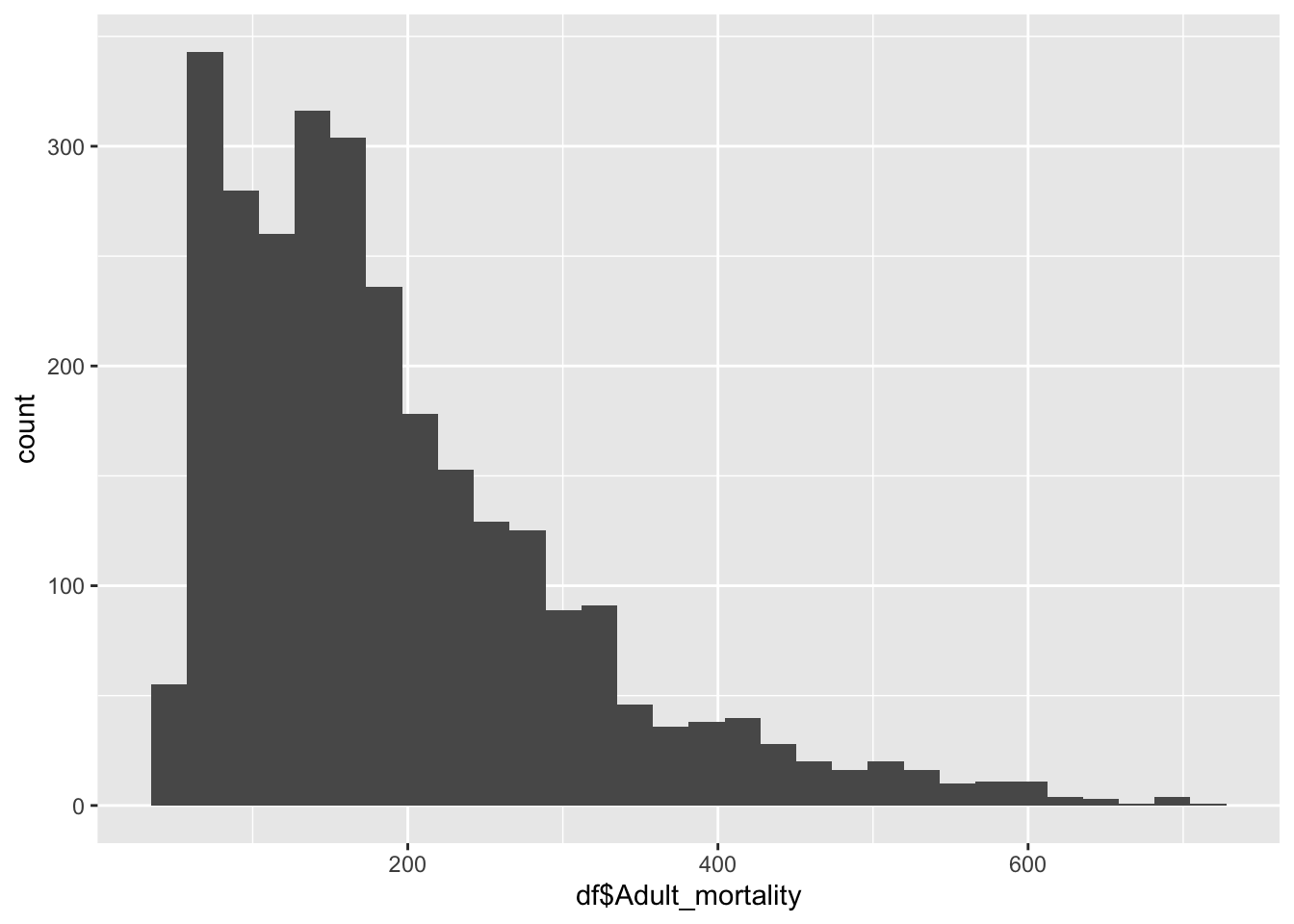

ggplot(df, aes(x=Adult_mortality, fill=Region)) +
    geom_histogram(bins=30, alpha=0.6, position="identity") +
    labs(title="Histogram of Adult_mortality by Region",
         x="Adult_mortality",
         y="Count") +
    theme_minimal()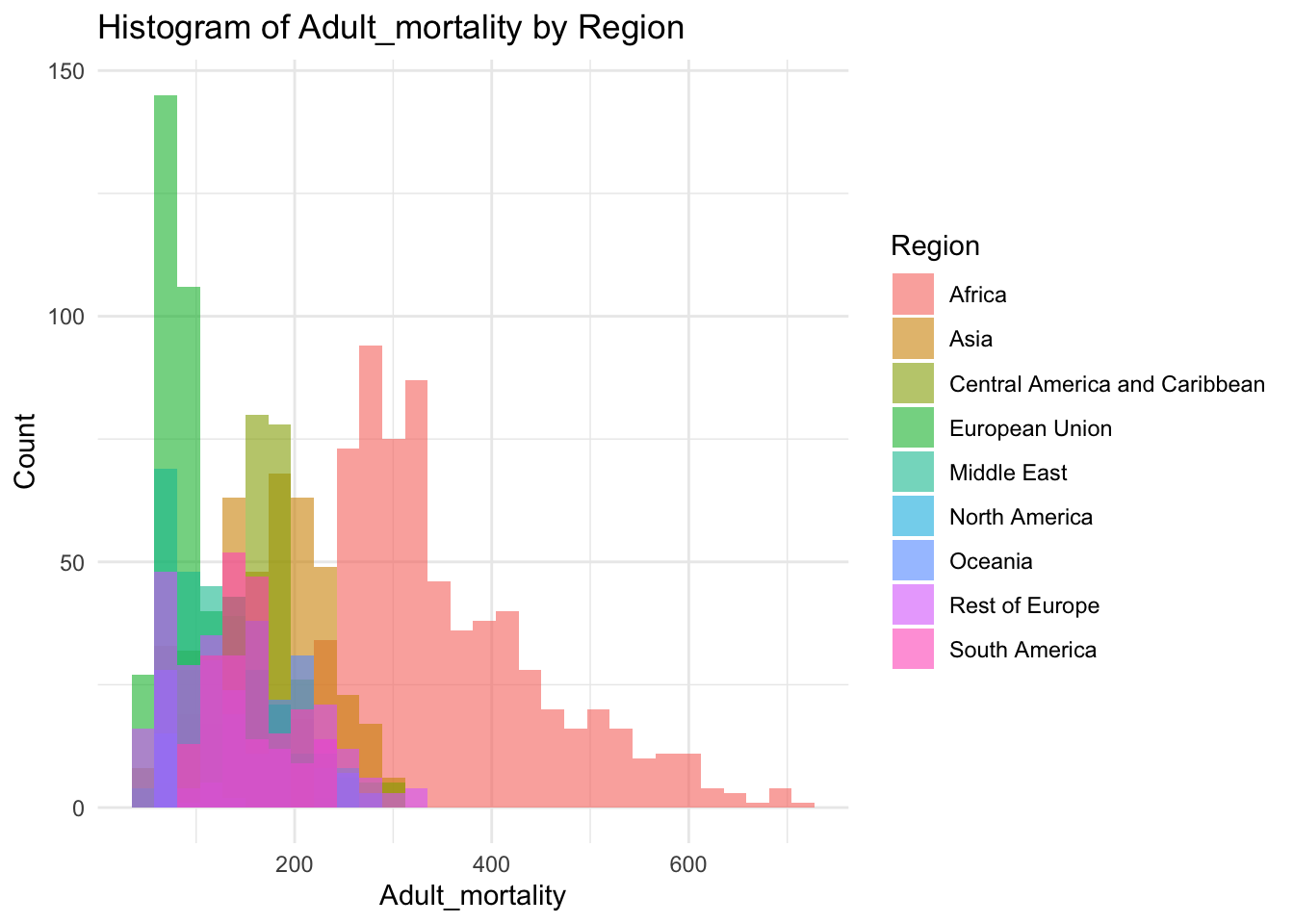

summary(df$Adult_mortality)

   Min. 1st Qu.  Median    Mean 3rd Qu.    Max. 
  49.38  106.91  163.84  192.25  246.79  719.36

Inference:

Adult mortality represents the adult deaths in the given country

Life Expectancy is not evenly distributed,

Adult mortality peaks ~164

The minimum is 49.38, the max is 719.36

Alcohol Consumption

df |>
ggplot() +
    geom_boxplot(aes(x=0, y=df$Alcohol_consumption))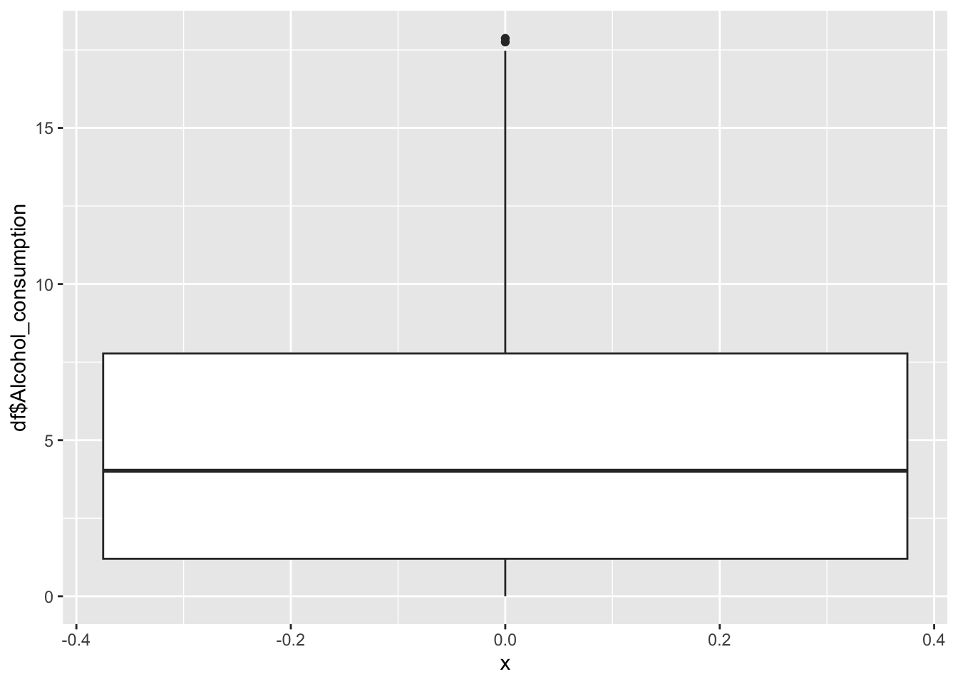

df |>
ggplot() +
    geom_histogram(aes(x=df$Alcohol_consumption), bins = 30)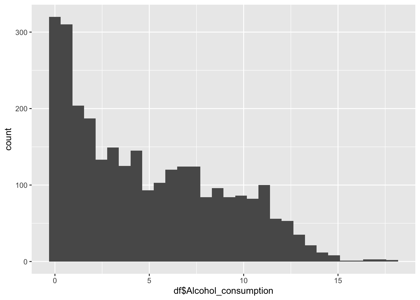

ggplot(df, aes(x=Alcohol_consumption, fill=Region)) +
    geom_histogram(bins=30, alpha=0.6, position="identity") +
    labs(title="Histogram of Alcohol_consumption by Region",
         x="Alcohol_consumption",
         y="Count") +
    theme_minimal()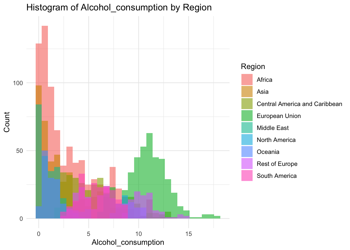

summary(df$Alcohol_consumption)

   Min. 1st Qu.  Median    Mean 3rd Qu.    Max. 
  0.000   1.200   4.020   4.821   7.777  17.870

Inference:

Alcohol consumption is recorded per capita (15+) consumption (in litres of pure alcohol)

Min is 0 litres

Max is 17.87

Alcohol consumption is not evenly distrusted.

Alcohol Consumption peaks at 0

$Hepatitis_B

df |>
ggplot() +
    geom_boxplot(aes(x=0, y=df$Hepatitis_B))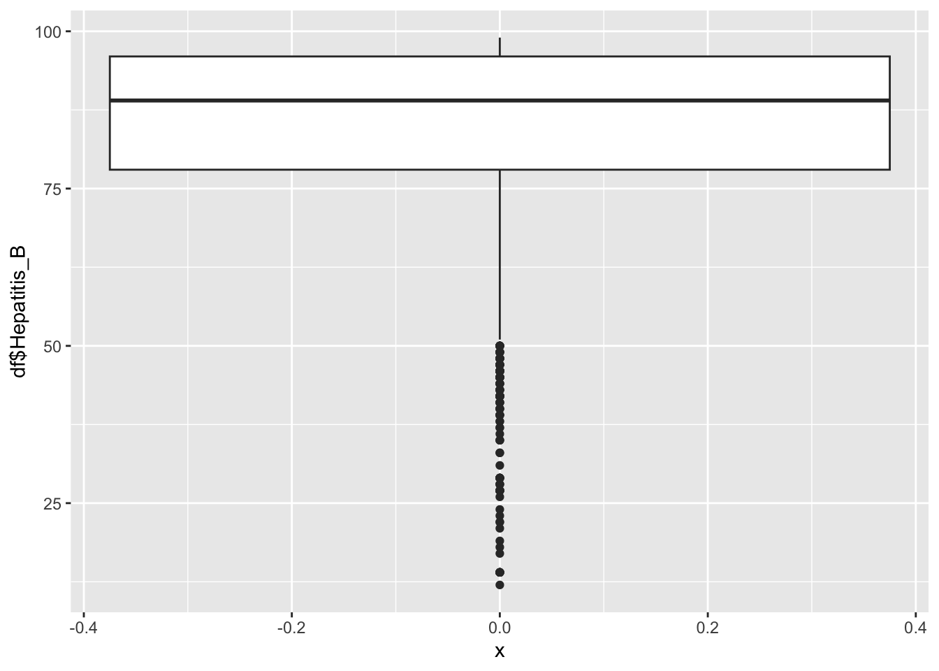

df |>
ggplot() +
    geom_histogram(aes(x=df$Hepatitis_B), bins = 30)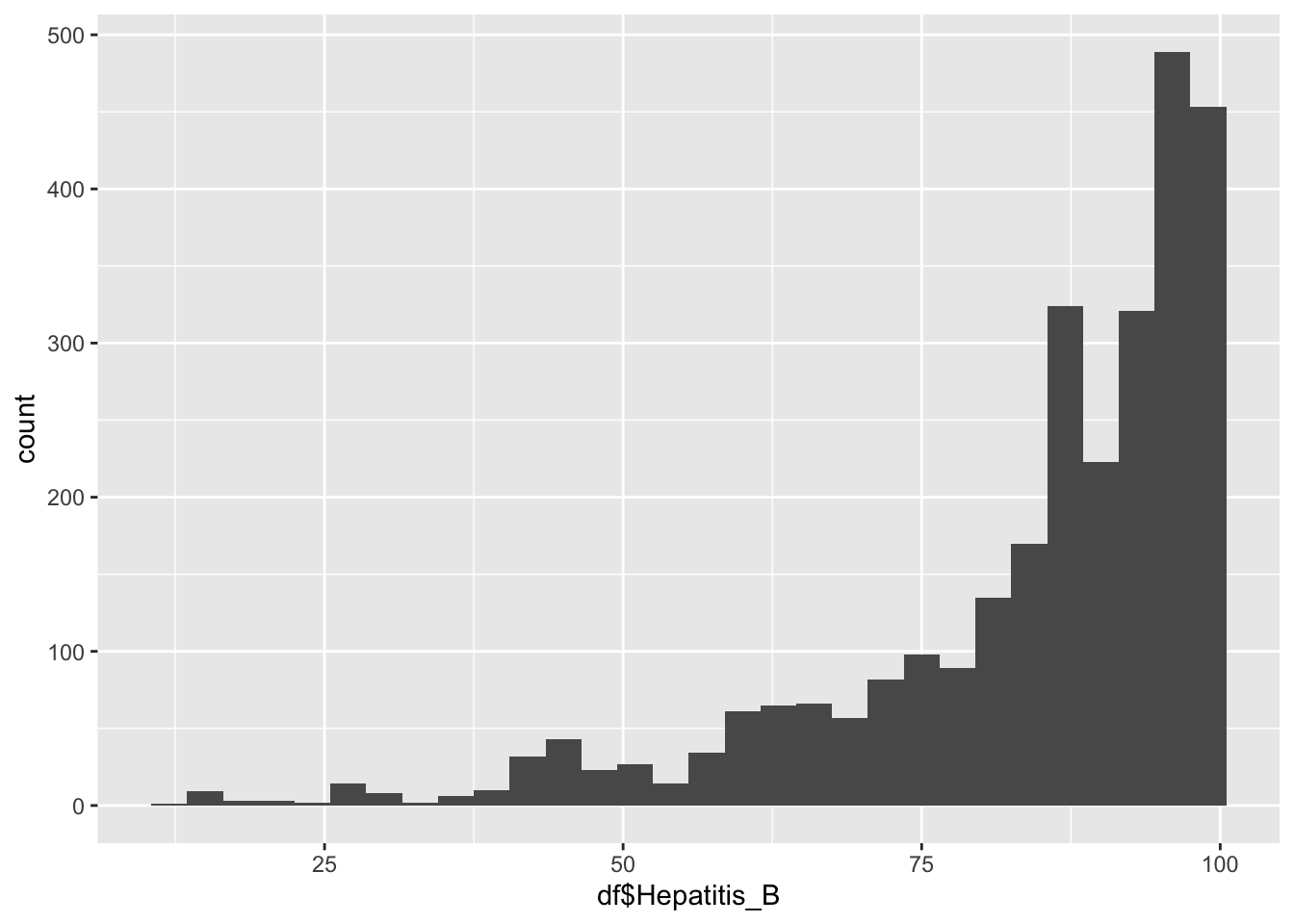

ggplot(df, aes(x=Hepatitis_B, fill=Region)) +
    geom_histogram(bins=30, alpha=0.6, position="identity") +
    labs(title="Histogram of Hepatitis_B by Region",
         x="Hepatitis_B",
         y="Count") +
    theme_minimal()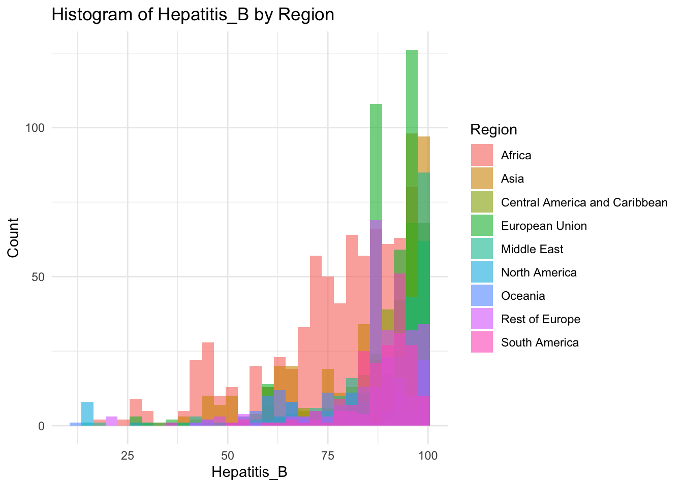

summary(df$Hepatitis_B)

   Min. 1st Qu.  Median    Mean 3rd Qu.    Max. 
  12.00   78.00   89.00   84.29   96.00   99.00

Hepatitis Inferences:

Hepatitis B represents the immunization coverage among 1-year olds(%)

It is not evenly distrusted

min: 12

Max 99.9

It peaks around 90%

Why is there a spike around 85?

That spike is due to the E.U.

Measles

df |>
ggplot() +
    geom_boxplot(aes(x=0, y=df$Measles))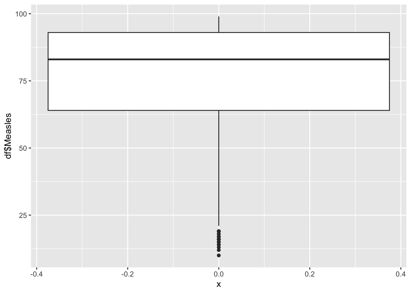

df |>
ggplot() +
    geom_histogram(aes(x=df$Measles), bins = 30)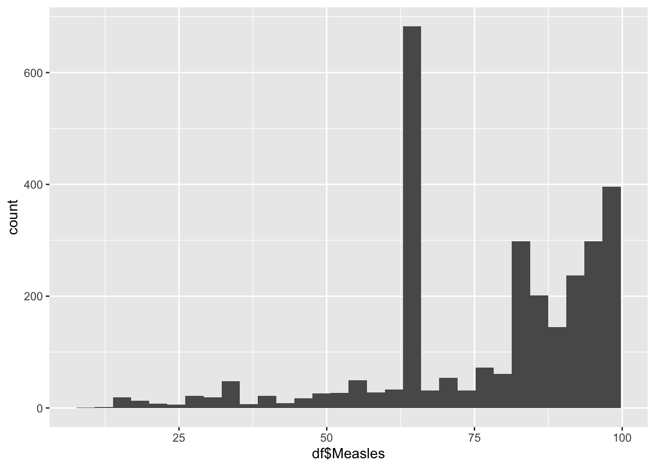

ggplot(df, aes(x=Measles, fill=Region)) +
    geom_histogram(bins=30, alpha=0.6, position="identity") +
    labs(title="Histogram of Measles by Region",
         x="Measles",
         y="Count") +
    theme_minimal()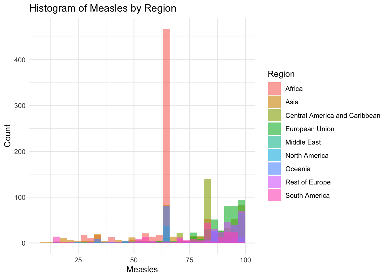

summary(df$Measles)

   Min. 1st Qu.  Median    Mean 3rd Qu.    Max. 
  10.00   64.00   83.00   77.34   93.00   99.00

Measles Influences:

Measles represents the percentage of 1 year olds who have been immunized

It is not evenly distrusted

Min 10

Max 99

It peaks around 62%

Why is there a spike around 62%?

Due to a large chunk of Africa

BMI

df |>
ggplot() +
    geom_boxplot(aes(x=0, y=df$BMI))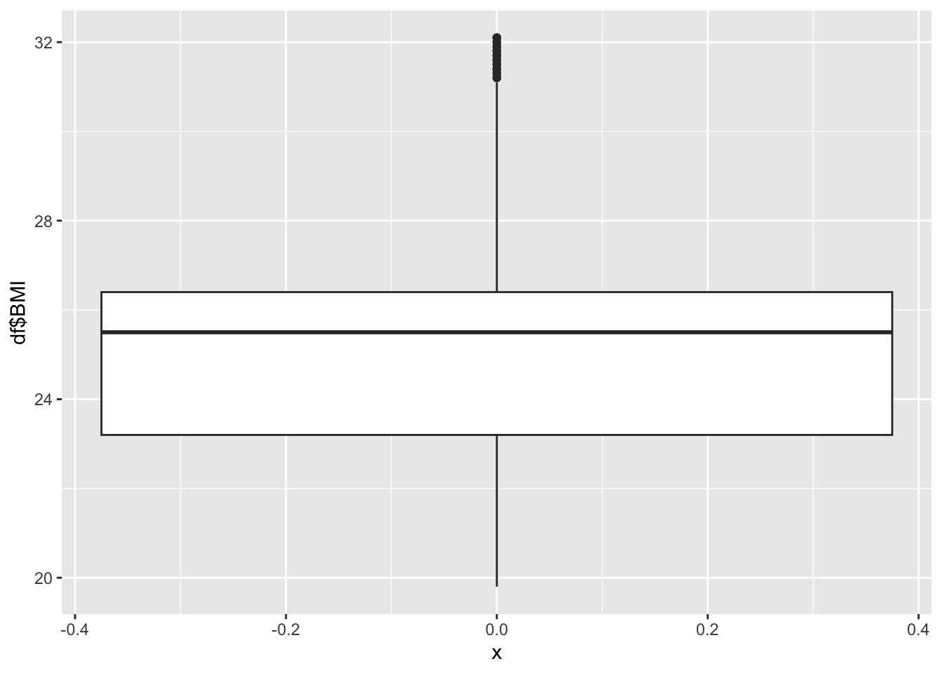

df |>
ggplot() +
    geom_histogram(aes(x=df$BMI), bins = 30)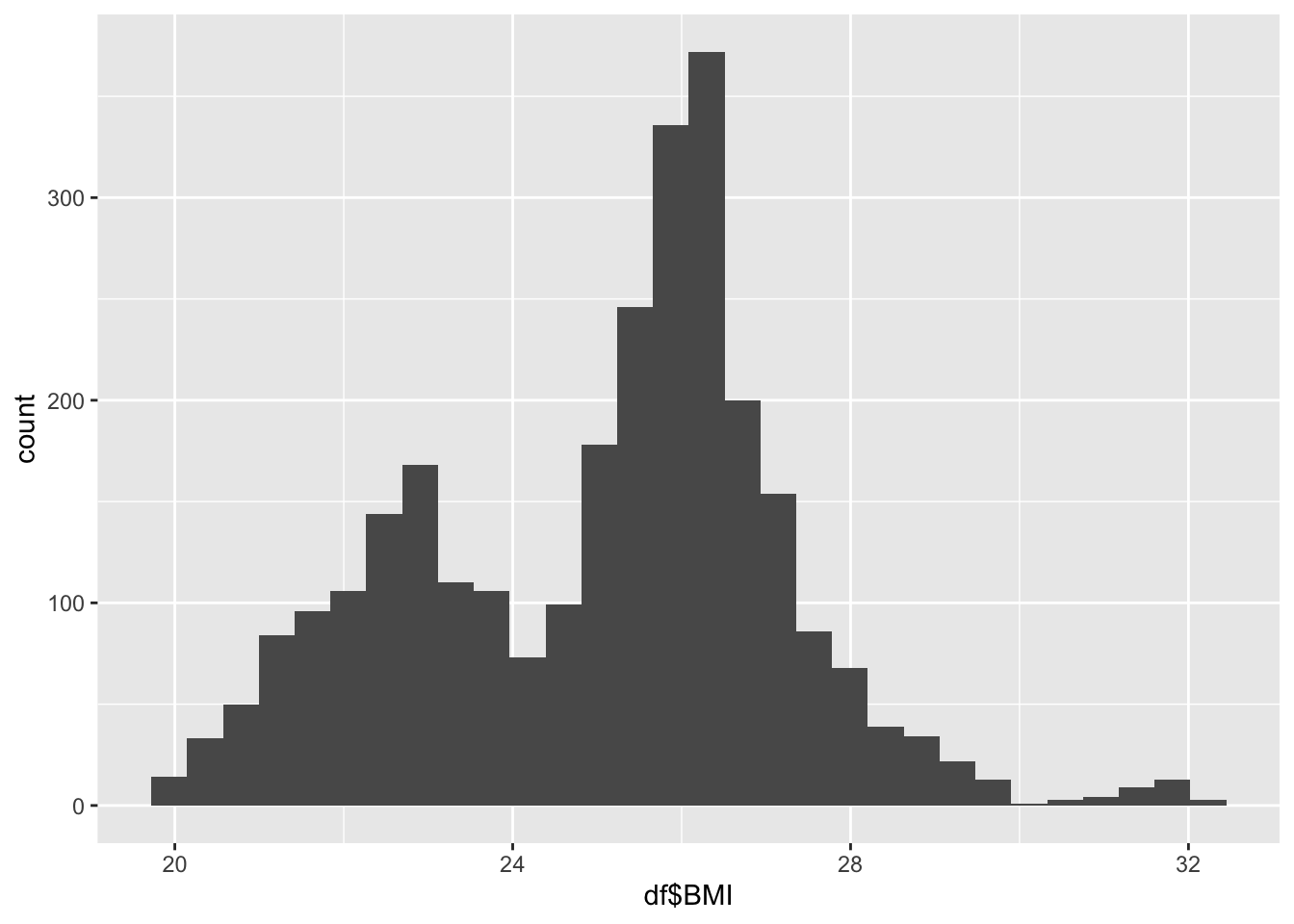

ggplot(df, aes(x=BMI, fill=Region)) +
    geom_histogram(bins=30, alpha=0.6, position="identity") +
    labs(title="Histogram of BMI by Region",
         x="BMI",
         y="Count") +
    theme_minimal()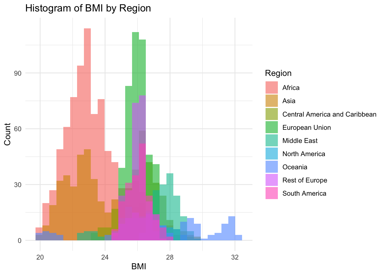

summary(df$BMI)

   Min. 1st Qu.  Median    Mean 3rd Qu.    Max. 
  19.80   23.20   25.50   25.03   26.40   32.10

BMI Inferences:

BMI represents the nutritional status of the adult population

It is not evenly distributed

Min 19

Max 32.10

Why is there two groups?

The two groups are two to African and Asia forming one peak, and Europe forming another peak

df |>
ggplot() +
    geom_boxplot(aes(x=0, y=df$Polio))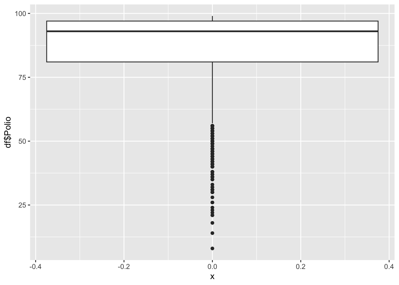

df |>
ggplot() +
    geom_histogram(aes(x=df$Polio), bins = 30)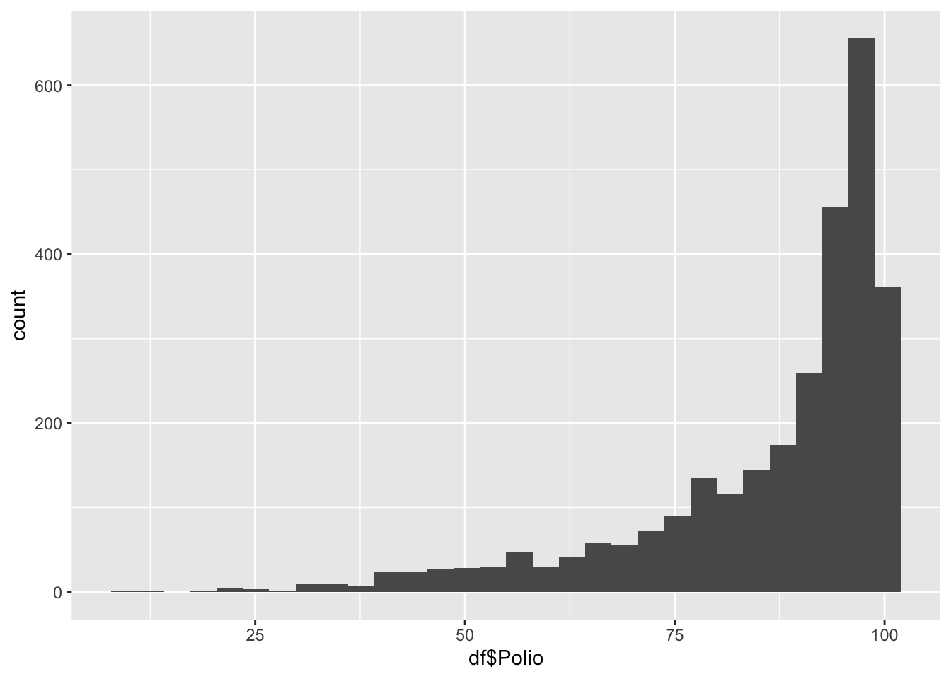

ggplot(df, aes(x=Polio, fill=Region)) +
    geom_histogram(bins=30, alpha=0.6, position="identity") +
    labs(title="Histogram of Polio by Region",
         x="Polio",
         y="Count") +
    theme_minimal()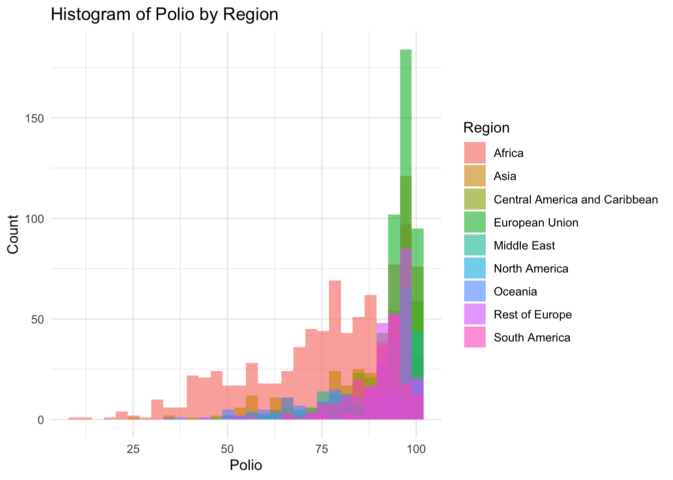

summary(df$Polio)

   Min. 1st Qu.  Median    Mean 3rd Qu.    Max. 
    8.0    81.0    93.0    86.5    97.0    99.0

Polio represents the percentage of one year-olds who were immunized for polio

Min: 8

Median 93.0

Max 99.0

Diphtheria

df |>
ggplot() +
    geom_boxplot(aes(x=0, y=df$Diphtheria))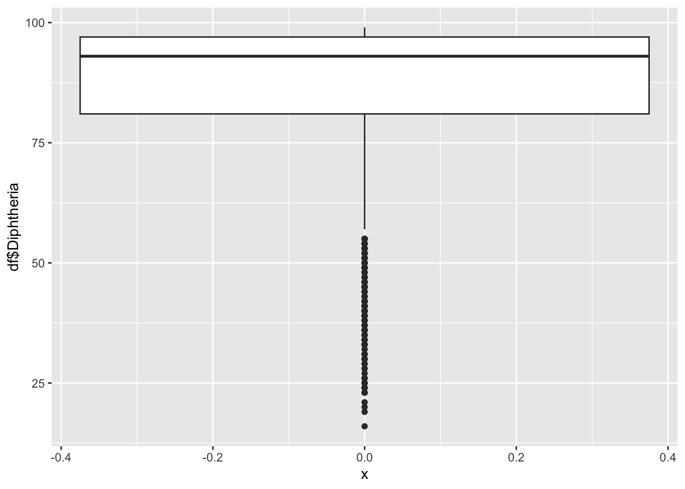

df |>
ggplot() +
    geom_histogram(aes(x=df$Diphtheria), bins = 30)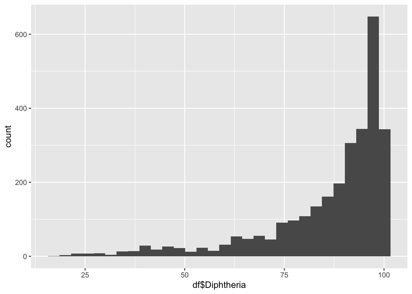

ggplot(df, aes(x=Diphtheria, fill=Region)) +
    geom_histogram(bins=30, alpha=0.6, position="identity") +
    labs(title="Histogram of Diphtheria by Region",
         x="Diphtheria",
         y="Count") +
    theme_minimal()

summary(df$Diphtheria)

   Min. 1st Qu.  Median    Mean 3rd Qu.    Max. 
  16.00   81.00   93.00   86.27   97.00   99.00

Polio represents the percentage of one year-olds who were immunized for Diphtheria

Min: 16

Median 93.0

Max 99.0

HIV

df |>
ggplot() +
    geom_boxplot(aes(x=0, y=df$Incidents_HIV))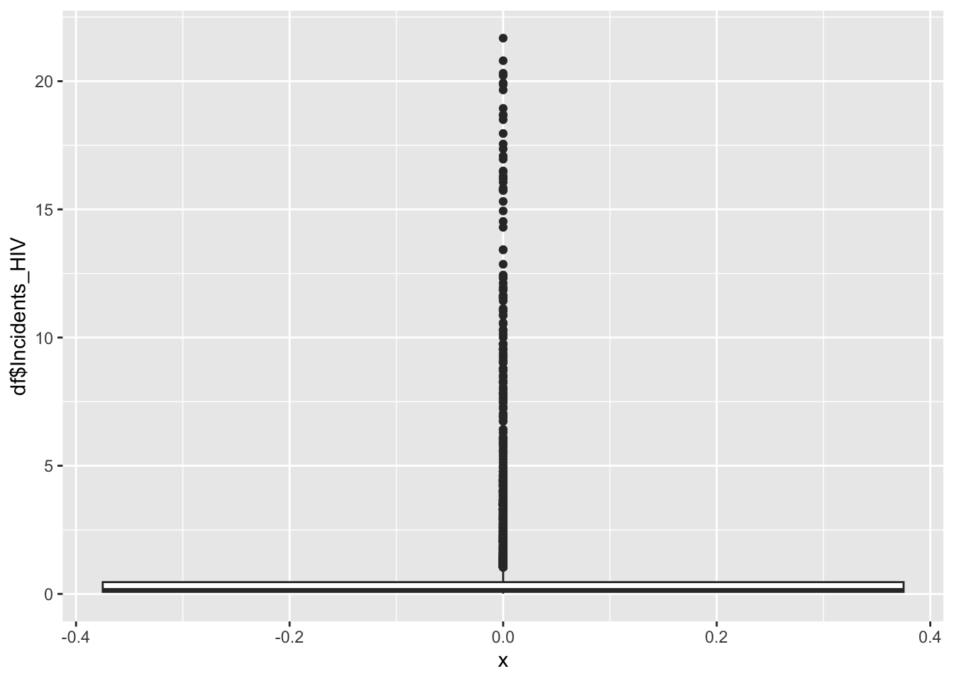

df |>
ggplot() +
    geom_histogram(aes(x=df$Incidents_HIV), bins = 30)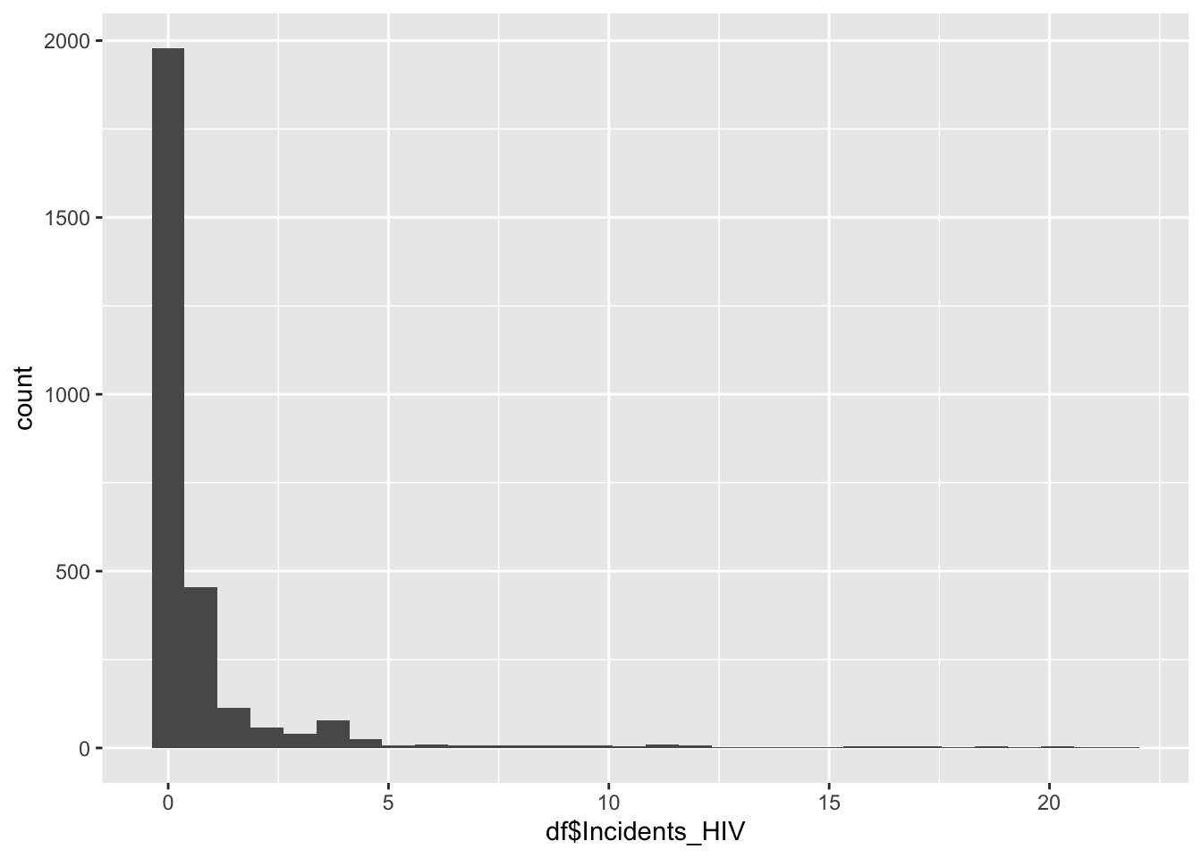

ggplot(df, aes(x=Incidents_HIV, fill=Region)) +
    geom_histogram(bins=30, alpha=0.6, position="identity") +
    labs(title="Histogram of Incidents_HIV by Region",
         x="Incidents_HIV",
         y="Count") +
    theme_minimal()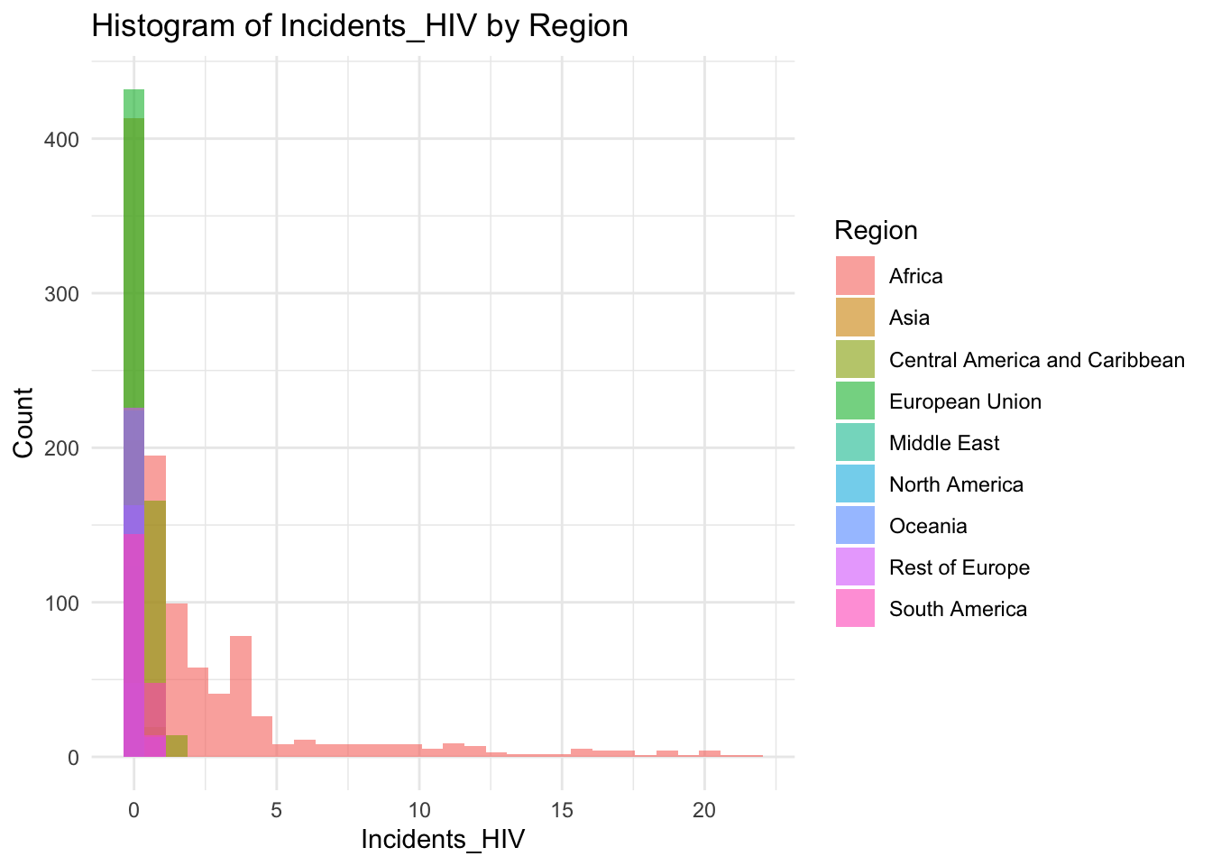

summary(df$Incidents_HIV)

   Min. 1st Qu.  Median    Mean 3rd Qu.    Max. 
 0.0100  0.0800  0.1500  0.8943  0.4600 21.6800

Min. 1st Qu.  Median    Mean 3rd Qu.    Max.  
0.0100  0.0800  0.1500  0.8943  0.4600 21.6800

Incidents_HIV represents the number of incidents of HIV per 1000 people

Min: 0.01

Median 0.15

Max:21.68

Most of the regions exist in the large spike at just after 0, with Africa making up the bulk of the rest of the graph, this is a possible explanation for Africa’s lower life expectancy

df |>
ggplot() +
    geom_boxplot(aes(x=0, y=df$GDP_per_capita))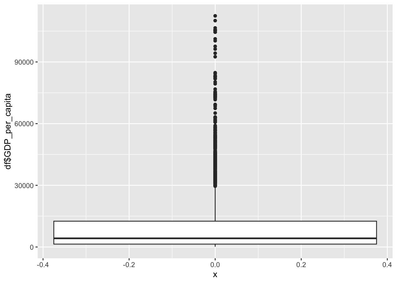

df |>
ggplot() +
    geom_histogram(aes(x=df$GDP_per_capita), bins = 30)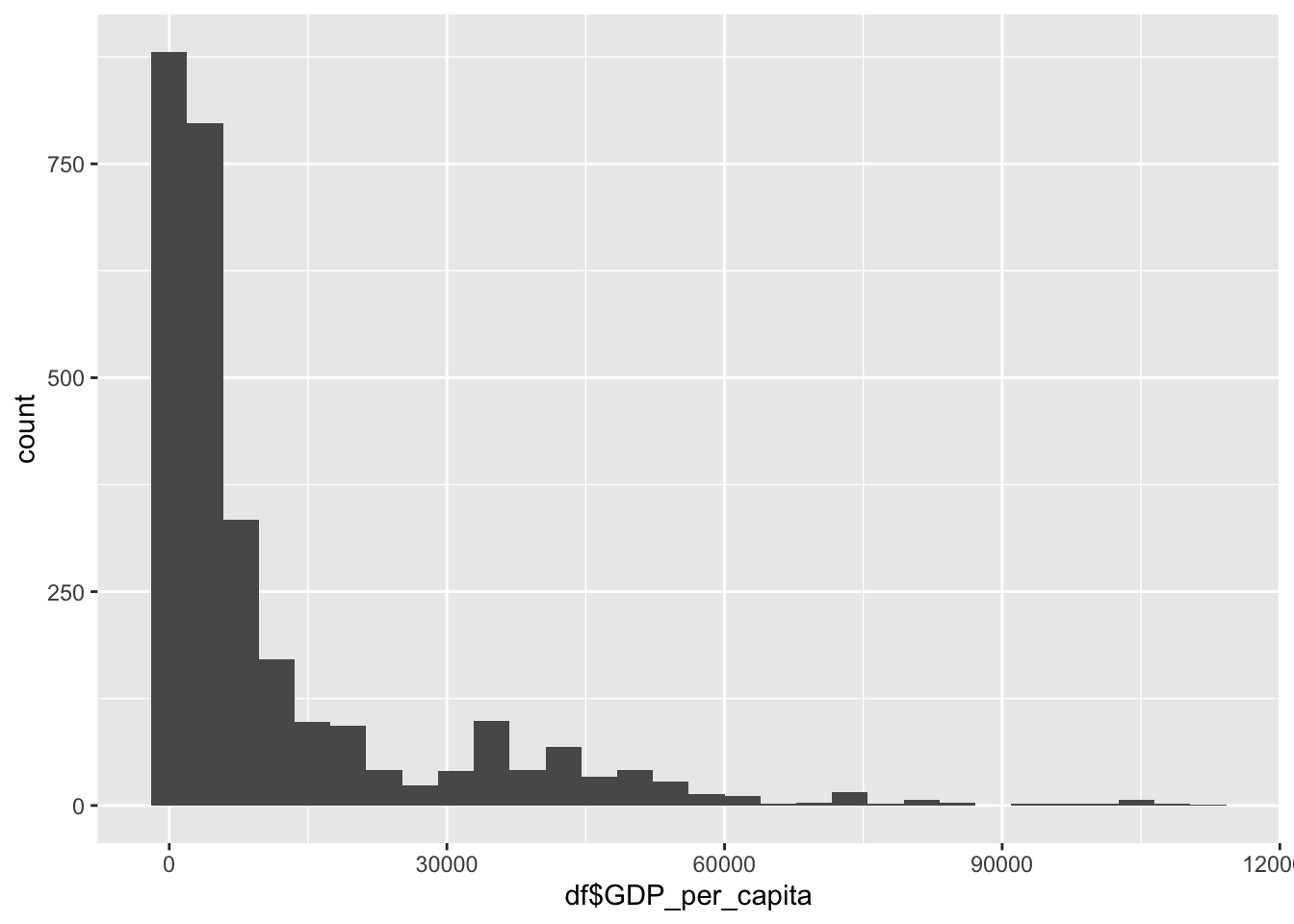

ggplot(df, aes(x=GDP_per_capita, fill=Region)) +
    geom_histogram(bins=30, alpha=0.6, position="identity") +
    labs(title="Histogram of GDP_per_capita by Region",
         x="GDP_per_capita",
         y="Count") +
    theme_minimal()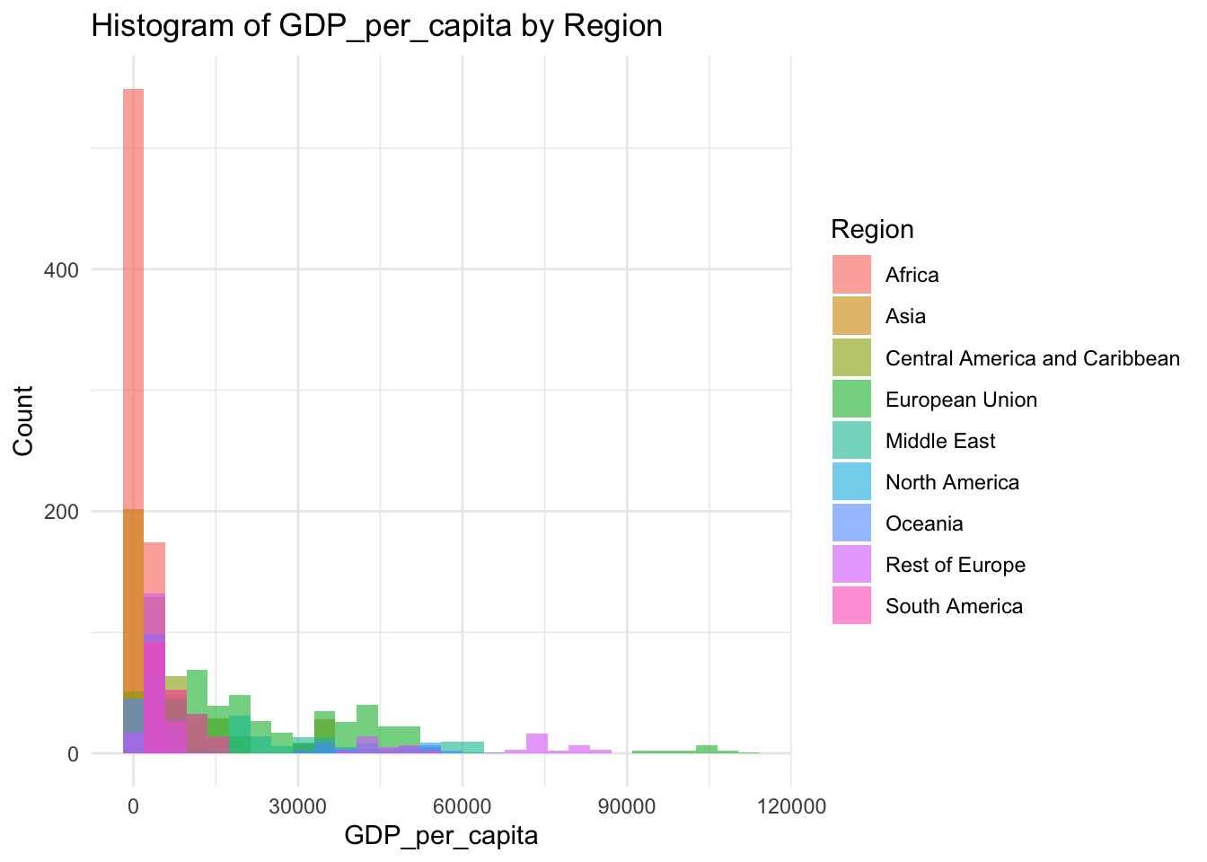

summary(df$GDP_per_capita)

   Min. 1st Qu.  Median    Mean 3rd Qu.    Max. 
    148    1416    4217   11541   12557  112418

GDP is a representation of the overall wealth of a country

Min:148

Median: 4217

Mean: 11541

Max: 112418

This variable has a very large range, with the majority of the world existing in the lower end of this scale.

Population

df |>
ggplot() +
    geom_boxplot(aes(x=0, y=df$Population_mln))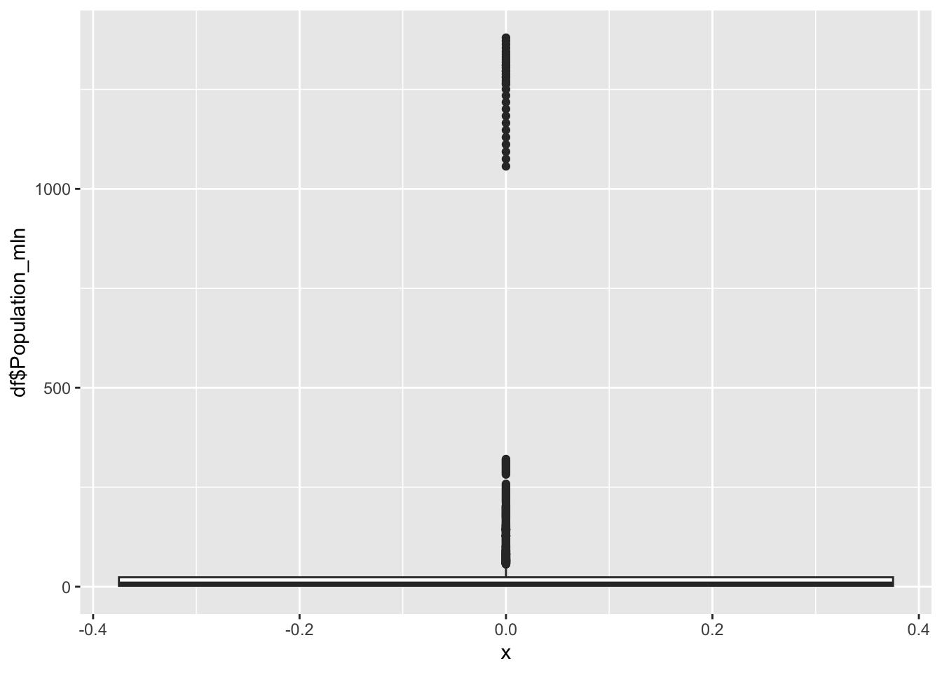

df |>
ggplot() +
    geom_histogram(aes(x=df$Population_mln), bins = 100)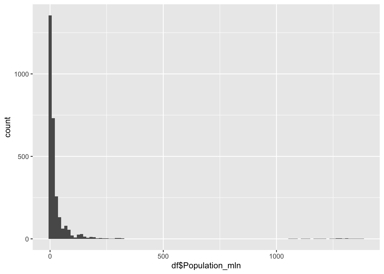

#re-do of the graph with xlim to exclude the outliers 
df |>
ggplot() +
    geom_histogram(aes(x=df$Population_mln), bins = 30) +
  xlim(0,350)

Warning: Removed 32 rows containing non-finite outside the scale range
(`stat_bin()`).

Warning: Removed 2 rows containing missing values or values outside the scale range
(`geom_bar()`).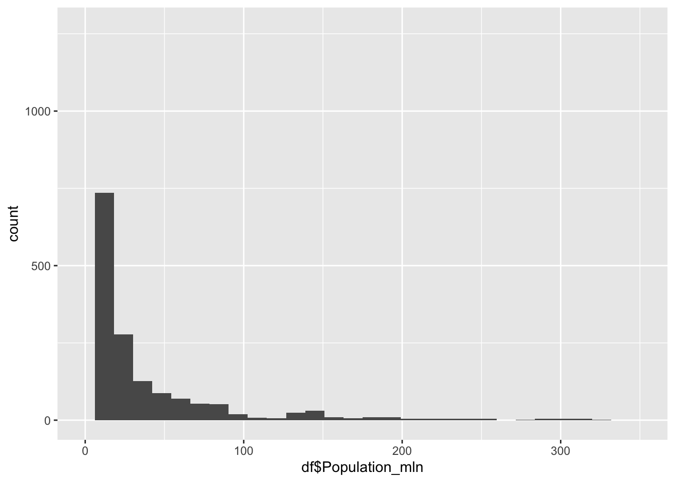

ggplot(df, aes(x=Population_mln, fill=Region)) +
    geom_histogram(bins=30, alpha=0.6, position="identity") +
    labs(title="Histogram of Population_mln by Region",
         x="Population_mln",
         y="Count") +
    theme_minimal()

summary(df$Population_mln)

    Min.  1st Qu.   Median     Mean  3rd Qu.     Max. 
   0.080    2.098    7.850   36.676   23.688 1379.860

Population represents the total number of people living within a nation, in the millions.

Min: 0.08

Median: 7.85

Mean: 36.676

Max: 1379.86

The outliers on the extreme edge are India and China.

Thinness 10 to 19

df |>
ggplot() +
    geom_boxplot(aes(x=0, y=df$Thinness_ten_nineteen_years))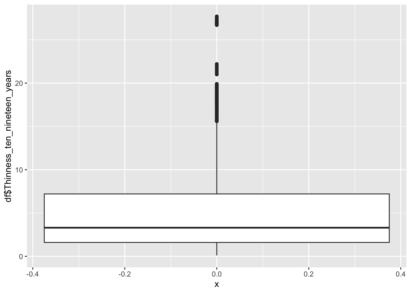

df |>
ggplot() +
    geom_histogram(aes(x=df$Thinness_ten_nineteen_years), bins = 30)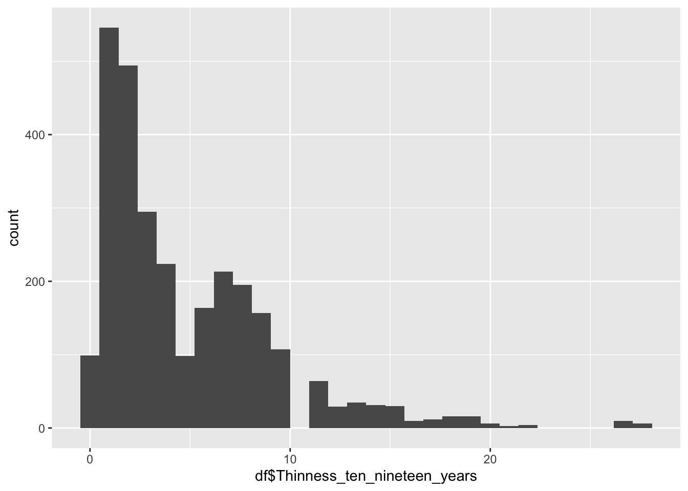

ggplot(df, aes(x=Thinness_ten_nineteen_years, fill=Region)) +
    geom_histogram(bins=30, alpha=0.6, position="identity") +
    labs(title="Histogram of Thinness_ten_nineteen_years by Region",
         x="Thinness_ten_nineteen_years",
         y="Count") +
    theme_minimal()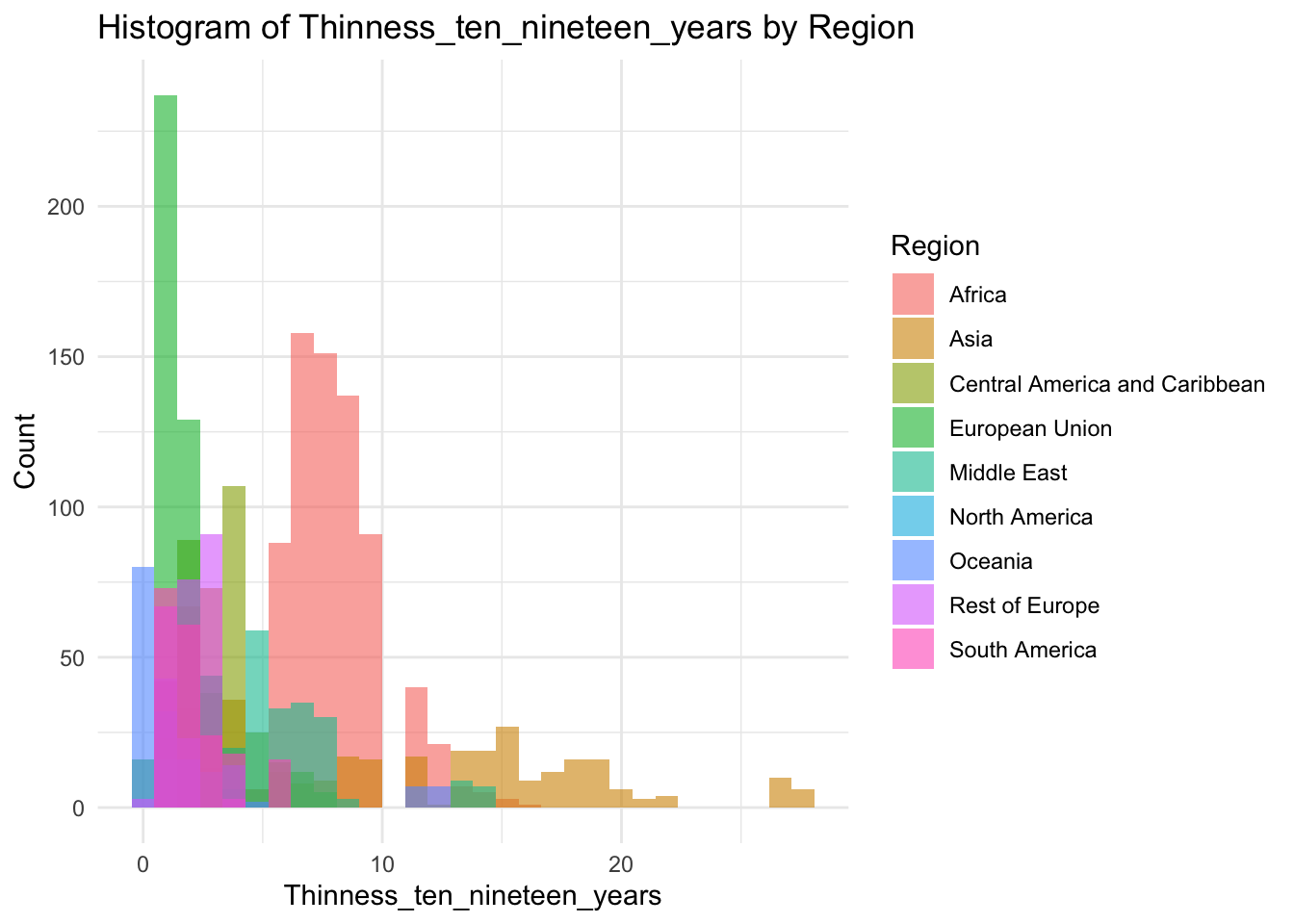

summary(df$Thinness_ten_nineteen_years)

   Min. 1st Qu.  Median    Mean 3rd Qu.    Max. 
  0.100   1.600   3.300   4.866   7.200  27.700

Thinness 10-19 represents the percentage of individuals in the age group who are “thin”

Min: 0.1

Median: 3.3

Mean 4.866

Max: 27.7

Why are there two groups?

The two peaks are formed by different regions, the first being Europe, the second being Africa.

df |>
ggplot() +
    geom_boxplot(aes(x=0, y=df$Thinness_five_nine_years))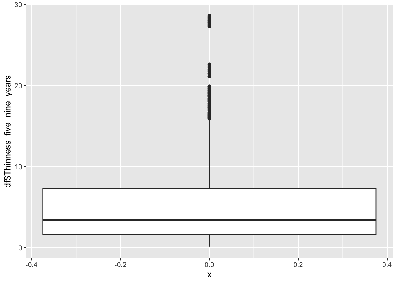

df |>
ggplot() +
    geom_histogram(aes(x=df$Thinness_five_nine_years), bins = 30)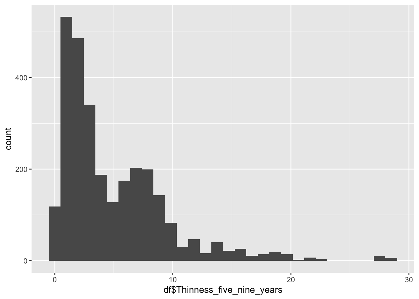

ggplot(df, aes(x=Thinness_five_nine_years, fill=Region)) +
    geom_histogram(bins=30, alpha=0.6, position="identity") +
    labs(title="Histogram of Thinness_five_nine_years by Region",
         x="Thinness_five_nine_years",
         y="Count") +
    theme_minimal()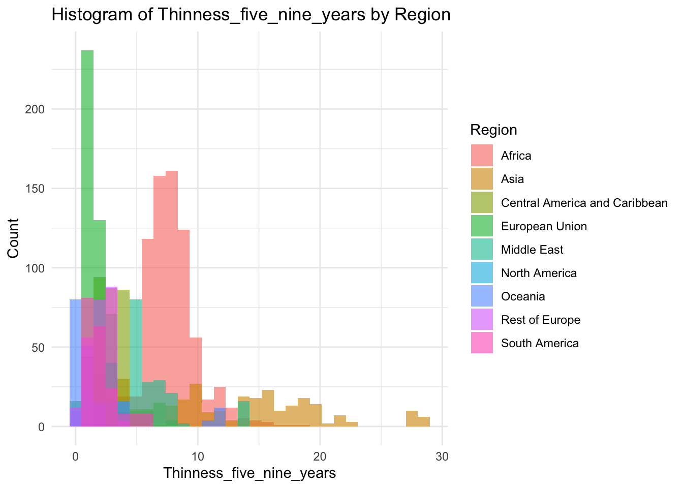

summary(df$Thinness_five_nine_years)

   Min. 1st Qu.  Median    Mean 3rd Qu.    Max. 
    0.1     1.6     3.4     4.9     7.3    28.6

Min: 0.1

Median:3.4

Mean:4.9

Max: 28.6

Why are there two groups?

Same as the 10-19 Thinness, Most of this graph is a mirror of the other Thinness graph.

df |>
ggplot() +
    geom_boxplot(aes(x=0, y=df$Schooling))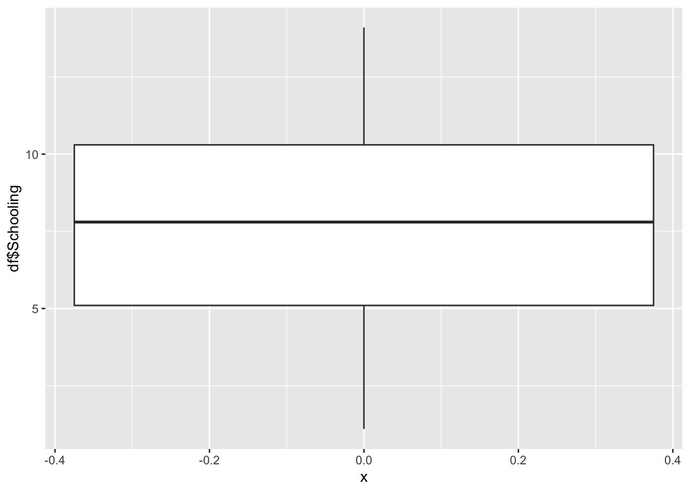

df |>
ggplot() +
    geom_histogram(aes(x=df$Schooling), bins = 30)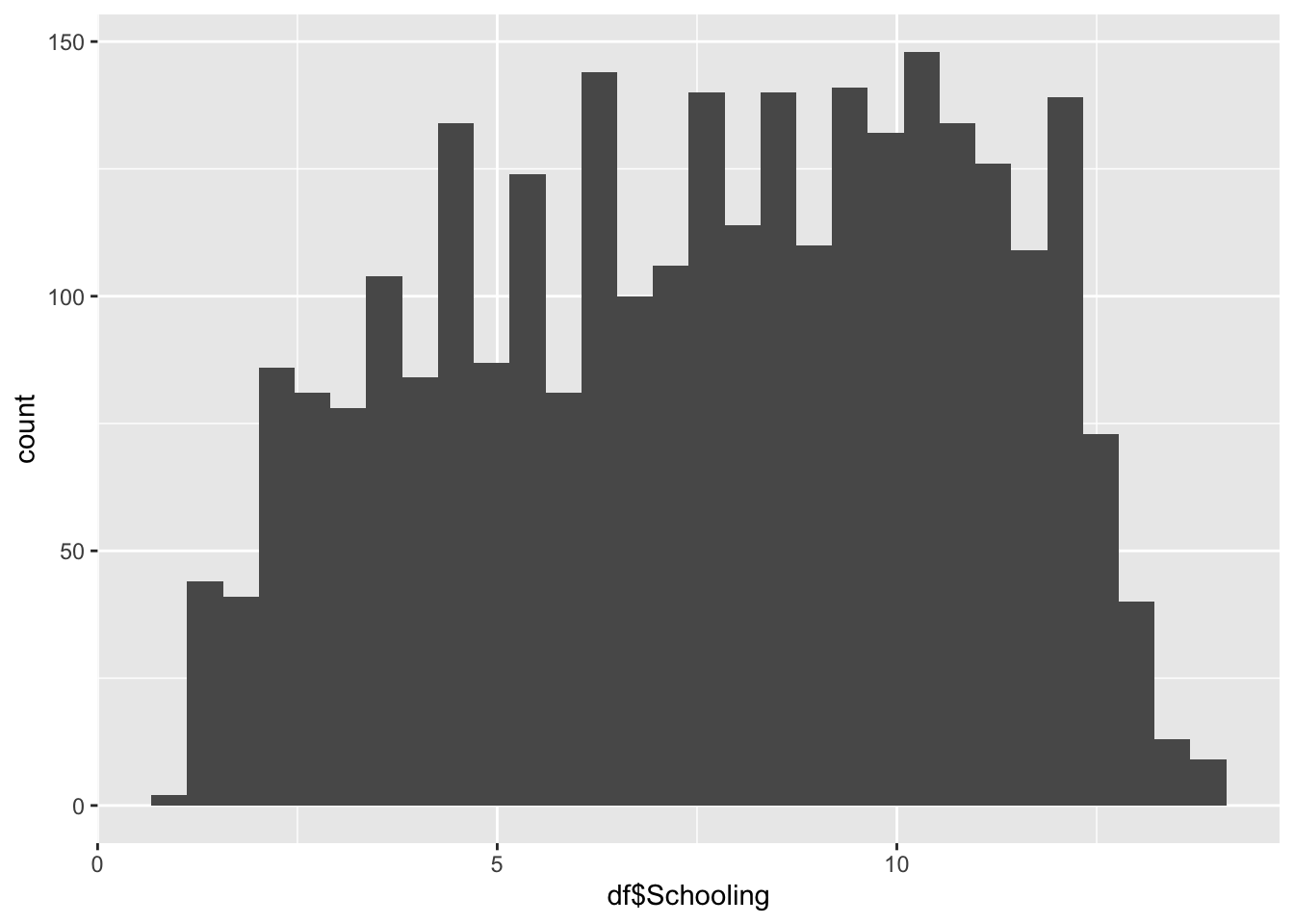

ggplot(df, aes(x=Schooling, fill=Region)) +
    geom_histogram(bins=30, alpha=0.6, position="identity") +
    labs(title="Histogram of Schooling by Region",
         x="Schooling",
         y="Count") +
    theme_minimal()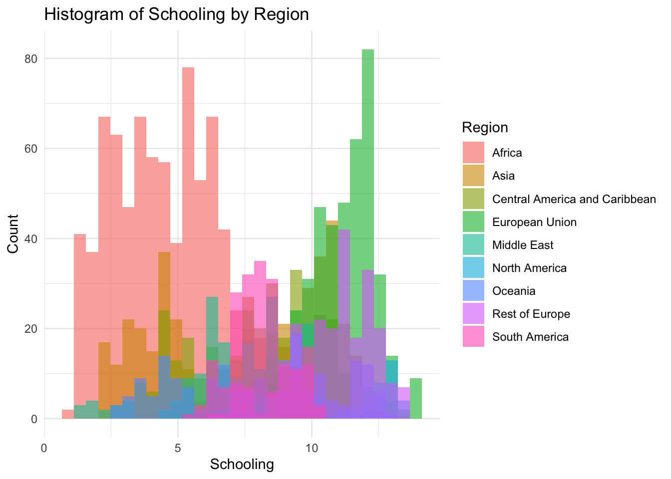

summary(df$Schooling)

   Min. 1st Qu.  Median    Mean 3rd Qu.    Max. 
  1.100   5.100   7.800   7.632  10.300  14.100

Schooling Represents the average years of schooling in the nation.

Min: 1.1

Median: 7.8

Mean: 7.632

Max: 14.1

Schooling is our most evenly distrusted graph so far.

4.3 Covariance Analysis

For Covariance Analysis we need a subset of the data that only has the numeric variables

Standardize the data

sdf <- df |>
  select(-Year, everything()) |>
  mutate(across(where(is.numeric), scale))

# Get only numeric data
numeric_data <- select_if(sdf, is.numeric)

cov_matrix <- cov(numeric_data)

print(cov_matrix)

                            Infant_deaths Under_five_deaths Adult_mortality
Infant_deaths                  1.00000000       0.985651346      0.79466086
Under_five_deaths              0.98565135       1.000000000      0.80236112
Adult_mortality                0.79466086       0.802361123      1.00000000
Alcohol_consumption           -0.45452615      -0.409367397     -0.24479376
Hepatitis_B                   -0.51256224      -0.507427407     -0.34488221
Measles                       -0.52628201      -0.512971742     -0.41615254
BMI                           -0.66198827      -0.665255042     -0.52286551
Polio                         -0.74079046      -0.742983474     -0.52422554
Diphtheria                    -0.72187465      -0.725355032     -0.51380270
Incidents_HIV                  0.34945826       0.369617726      0.69911938
GDP_per_capita                -0.51228611      -0.469681668     -0.51012141
Population_mln                 0.00762199      -0.005234231     -0.05384768
Thinness_ten_nineteen_years    0.49119174       0.466978458      0.38214030
Thinness_five_nine_years       0.47763934       0.450755699      0.37979229
Schooling                     -0.78851253      -0.773195983     -0.58103548
Life_expectancy               -0.92003192      -0.920419134     -0.94536036
                            Alcohol_consumption Hepatitis_B     Measles
Infant_deaths                       -0.45452615 -0.51256224 -0.52628201
Under_five_deaths                   -0.40936740 -0.50742741 -0.51297174
Adult_mortality                     -0.24479376 -0.34488221 -0.41615254
Alcohol_consumption                  1.00000000  0.16843582  0.31860293
Hepatitis_B                          0.16843582  1.00000000  0.42916779
Measles                              0.31860293  0.42916779  1.00000000
BMI                                  0.28403195  0.34542091  0.41632141
Polio                                0.30192623  0.72434526  0.51409629
Diphtheria                           0.29901592  0.76178009  0.49405877
Incidents_HIV                       -0.03411801 -0.07578195 -0.15058000
GDP_per_capita                       0.44396595  0.15937504  0.31372372
Population_mln                      -0.03911866 -0.08239640 -0.09822189
Thinness_ten_nineteen_years         -0.44636618 -0.20845350 -0.34070533
Thinness_five_nine_years            -0.43302972 -0.21379442 -0.36696995
Schooling                            0.61572804  0.34764345  0.49839128
Life_expectancy                      0.39915911  0.41780443  0.49001859
                                   BMI       Polio  Diphtheria Incidents_HIV
Infant_deaths               -0.6619883 -0.74079046 -0.72187465    0.34945826
Under_five_deaths           -0.6652550 -0.74298347 -0.72535503    0.36961773
Adult_mortality             -0.5228655 -0.52422554 -0.51380270    0.69911938
Alcohol_consumption          0.2840319  0.30192623  0.29901592   -0.03411801
Hepatitis_B                  0.3454209  0.72434526  0.76178009   -0.07578195
Measles                      0.4163214  0.51409629  0.49405877   -0.15058000
BMI                          1.0000000  0.45720604  0.42650090   -0.16114208
Polio                        0.4572060  1.00000000  0.95317790   -0.14795220
Diphtheria                   0.4265009  0.95317790  1.00000000   -0.14693191
Incidents_HIV               -0.1611421 -0.14795220 -0.14693191    1.00000000
GDP_per_capita               0.3361796  0.31378567  0.31332094   -0.16958972
Population_mln              -0.1664820 -0.03348589 -0.02733598   -0.05803971
Thinness_ten_nineteen_years -0.5964833 -0.31268545 -0.30446625    0.18876454
Thinness_five_nine_years    -0.5991122 -0.30699811 -0.29559745    0.19384734
Schooling                    0.6354752  0.55276511  0.53562097   -0.20124620
Life_expectancy              0.5984233  0.64121746  0.62754139   -0.55302746
                            GDP_per_capita Population_mln
Infant_deaths                  -0.51228611    0.007621990
Under_five_deaths              -0.46968167   -0.005234231
Adult_mortality                -0.51012141   -0.053847680
Alcohol_consumption             0.44396595   -0.039118659
Hepatitis_B                     0.15937504   -0.082396398
Measles                         0.31372372   -0.098221891
BMI                             0.33617960   -0.166482004
Polio                           0.31378567   -0.033485888
Diphtheria                      0.31332094   -0.027335977
Incidents_HIV                  -0.16958972   -0.058039708
GDP_per_capita                  1.00000000   -0.040838867
Population_mln                 -0.04083887    1.000000000
Thinness_ten_nineteen_years    -0.37526974    0.256322009
Thinness_five_nine_years       -0.38103211    0.258485836
Schooling                       0.58062592   -0.033561816
Life_expectancy                 0.58308972    0.026297880
                            Thinness_ten_nineteen_years
Infant_deaths                                 0.4911917
Under_five_deaths                             0.4669785
Adult_mortality                               0.3821403
Alcohol_consumption                          -0.4463662
Hepatitis_B                                  -0.2084535
Measles                                      -0.3407053
BMI                                          -0.5964833
Polio                                        -0.3126855
Diphtheria                                   -0.3044662
Incidents_HIV                                 0.1887645
GDP_per_capita                               -0.3752697
Population_mln                                0.2563220
Thinness_ten_nineteen_years                   1.0000000
Thinness_five_nine_years                      0.9387571
Schooling                                    -0.5714852
Life_expectancy                              -0.4678245
                            Thinness_five_nine_years   Schooling
Infant_deaths                              0.4776393 -0.78851253
Under_five_deaths                          0.4507557 -0.77319598
Adult_mortality                            0.3797923 -0.58103548
Alcohol_consumption                       -0.4330297  0.61572804
Hepatitis_B                               -0.2137944  0.34764345
Measles                                   -0.3669700  0.49839128
BMI                                       -0.5991122  0.63547517
Polio                                     -0.3069981  0.55276511
Diphtheria                                -0.2955975  0.53562097
Incidents_HIV                              0.1938473 -0.20124620
GDP_per_capita                            -0.3810321  0.58062592
Population_mln                             0.2584858 -0.03356182
Thinness_ten_nineteen_years                0.9387571 -0.57148516
Thinness_five_nine_years                   1.0000000 -0.55137635
Schooling                                 -0.5513764  1.00000000
Life_expectancy                           -0.4581662  0.73248447
                            Life_expectancy
Infant_deaths                   -0.92003192
Under_five_deaths               -0.92041913
Adult_mortality                 -0.94536036
Alcohol_consumption              0.39915911
Hepatitis_B                      0.41780443
Measles                          0.49001859
BMI                              0.59842332
Polio                            0.64121746
Diphtheria                       0.62754139
Incidents_HIV                   -0.55302746
GDP_per_capita                   0.58308972
Population_mln                   0.02629788
Thinness_ten_nineteen_years     -0.46782450
Thinness_five_nine_years        -0.45816623
Schooling                        0.73248447
Life_expectancy                  1.00000000

Life Expectancy:

covariance_plot("Life_expectancy", "Adult_mortality", df, sdf)

Warning: `aes_string()` was deprecated in ggplot2 3.0.0.
ℹ Please use tidy evaluation idioms with `aes()`.
ℹ See also `vignette("ggplot2-in-packages")` for more information.

Warning in geom_text(aes(label = paste("Covariance:", round(cov(std_data_frame[[y_val]], : All aesthetics have length 1, but the data has 2864 rows.
ℹ Please consider using `annotate()` or provide this layer with data containing
  a single row.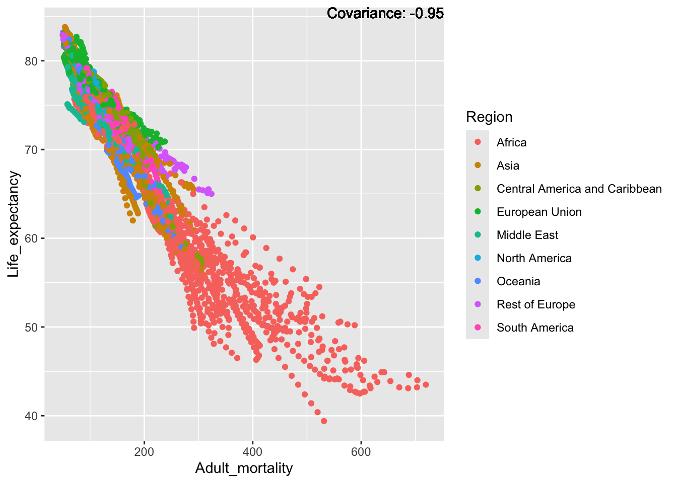

covariance_plot("Life_expectancy", "Infant_deaths", df, sdf)

Warning in geom_text(aes(label = paste("Covariance:", round(cov(std_data_frame[[y_val]], : All aesthetics have length 1, but the data has 2864 rows.
ℹ Please consider using `annotate()` or provide this layer with data containing
  a single row.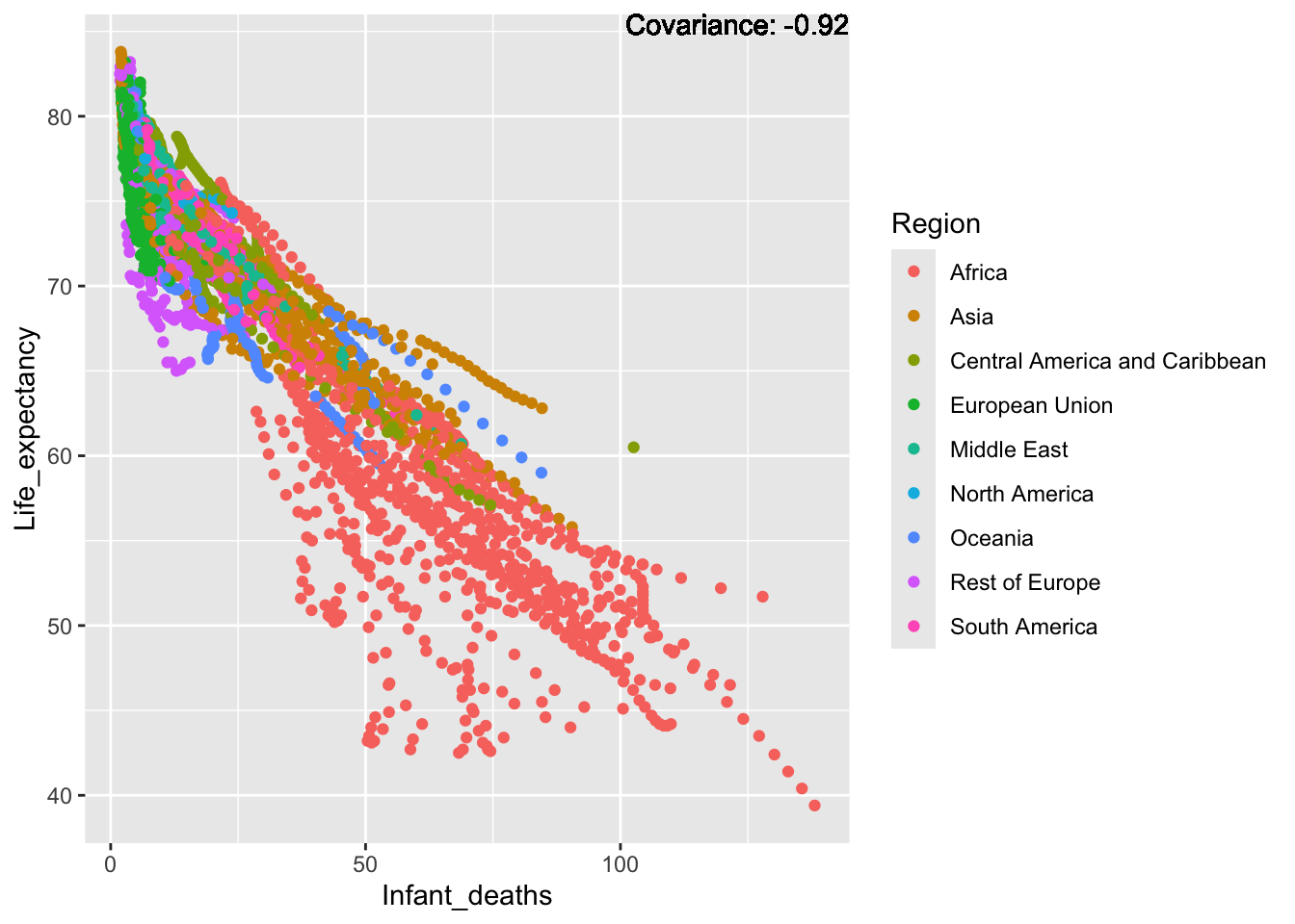

covariance_plot("Life_expectancy", "Under_five_deaths", df, sdf)

Warning in geom_text(aes(label = paste("Covariance:", round(cov(std_data_frame[[y_val]], : All aesthetics have length 1, but the data has 2864 rows.
ℹ Please consider using `annotate()` or provide this layer with data containing
  a single row.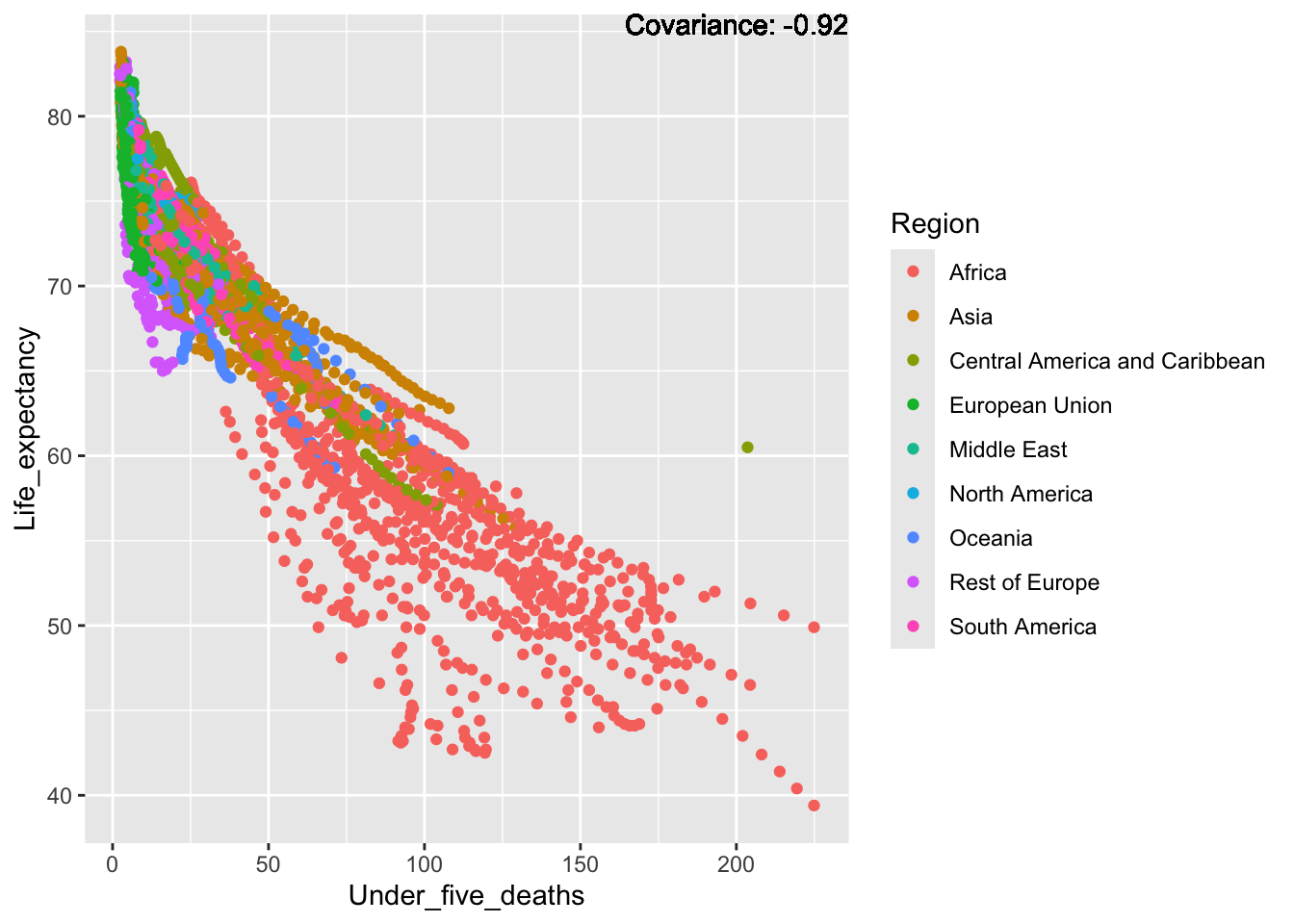

covariance_plot("Life_expectancy", "Alcohol_consumption", df, sdf)

Warning in geom_text(aes(label = paste("Covariance:", round(cov(std_data_frame[[y_val]], : All aesthetics have length 1, but the data has 2864 rows.
ℹ Please consider using `annotate()` or provide this layer with data containing
  a single row.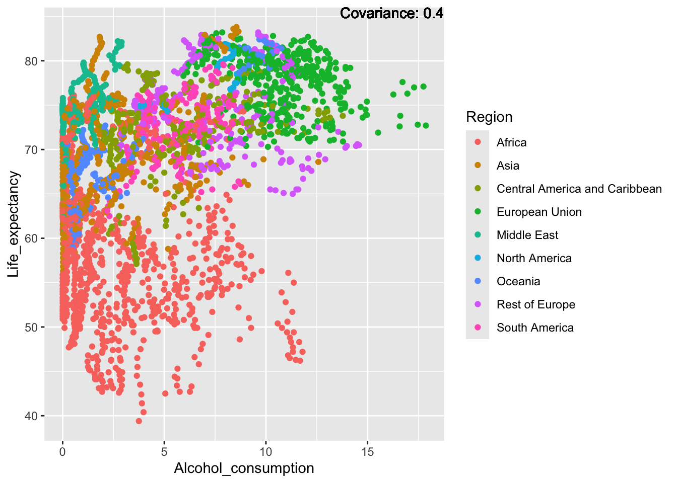

covariance_plot("Life_expectancy", "Hepatitis_B", df, sdf)

Warning in geom_text(aes(label = paste("Covariance:", round(cov(std_data_frame[[y_val]], : All aesthetics have length 1, but the data has 2864 rows.
ℹ Please consider using `annotate()` or provide this layer with data containing
  a single row.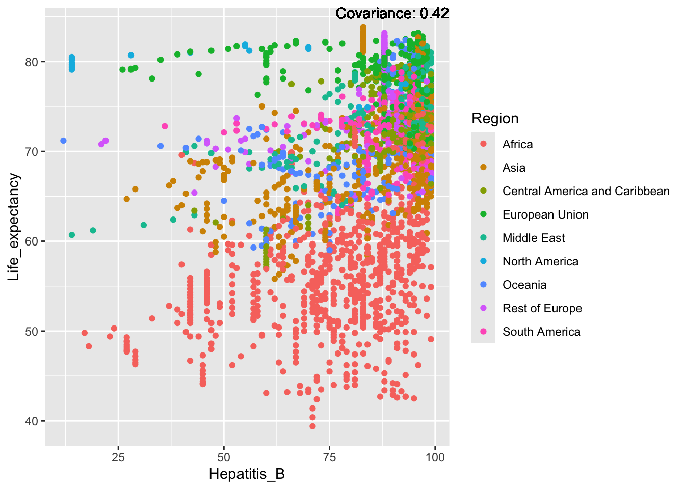

covariance_plot("Life_expectancy", "Measles", df, sdf)

Warning in geom_text(aes(label = paste("Covariance:", round(cov(std_data_frame[[y_val]], : All aesthetics have length 1, but the data has 2864 rows.
ℹ Please consider using `annotate()` or provide this layer with data containing
  a single row.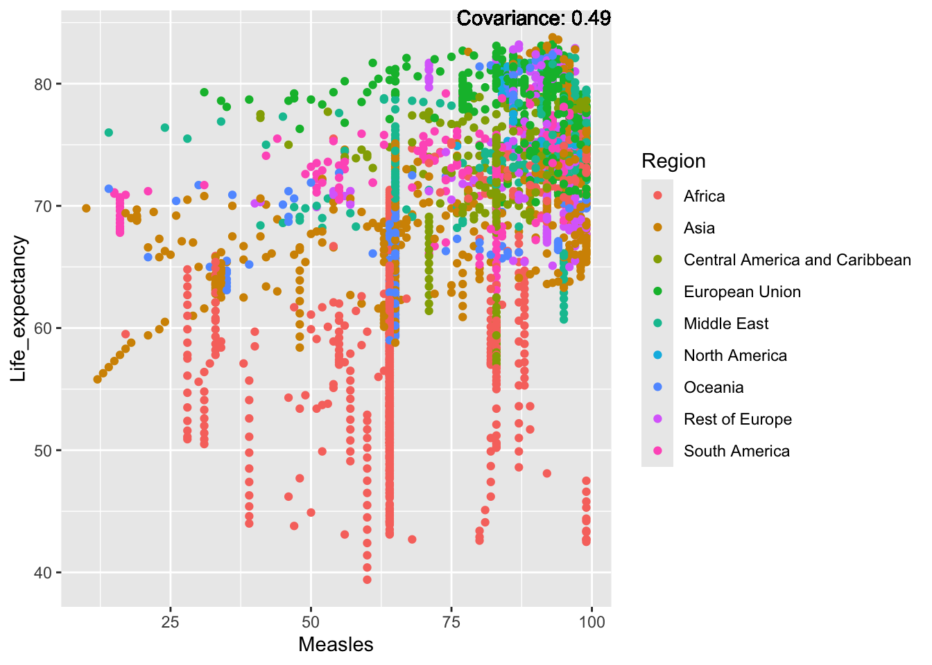

covariance_plot("Life_expectancy", "BMI", df, sdf)

Warning in geom_text(aes(label = paste("Covariance:", round(cov(std_data_frame[[y_val]], : All aesthetics have length 1, but the data has 2864 rows.
ℹ Please consider using `annotate()` or provide this layer with data containing
  a single row.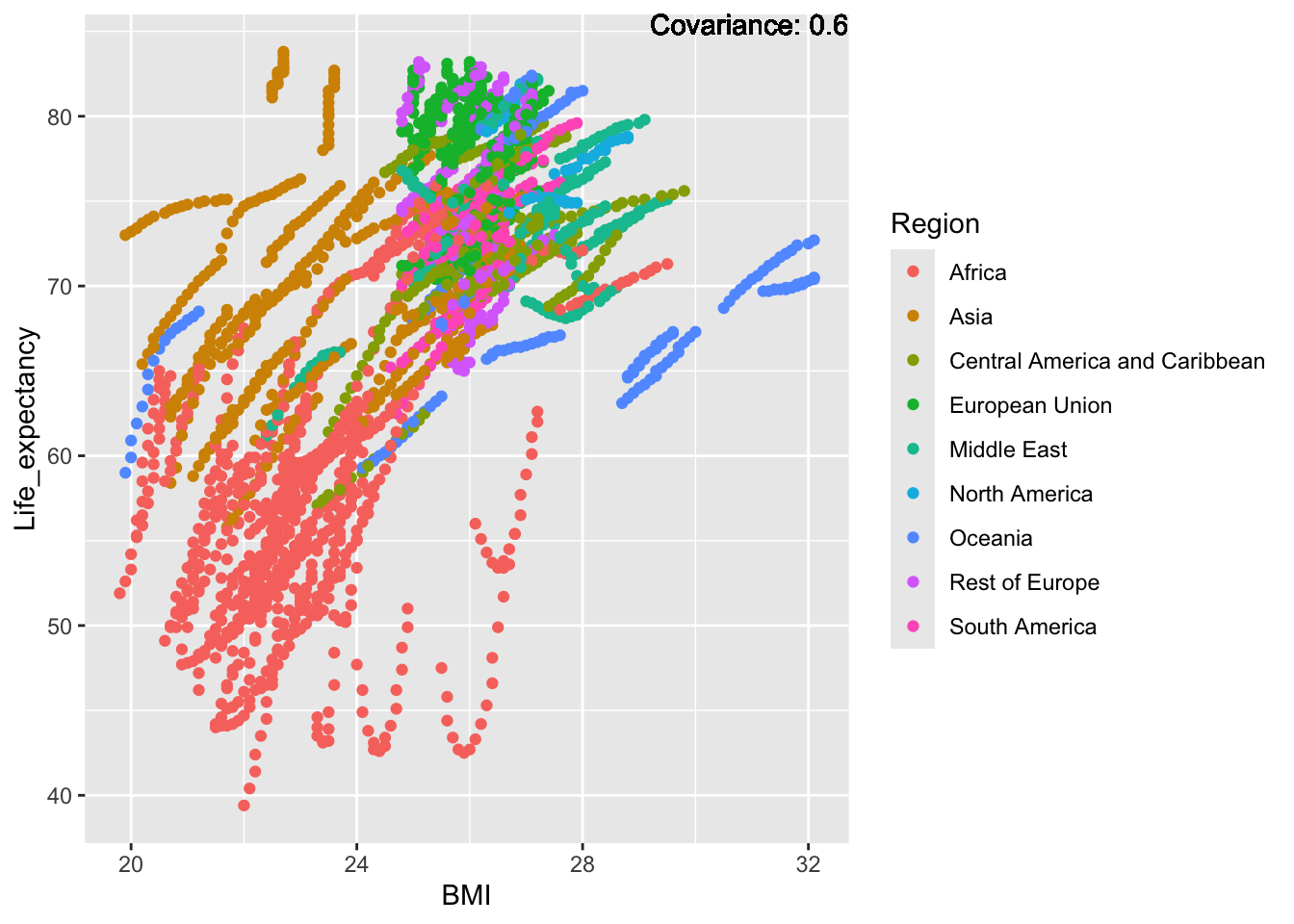

covariance_plot("Life_expectancy", "Polio", df, sdf)

Warning in geom_text(aes(label = paste("Covariance:", round(cov(std_data_frame[[y_val]], : All aesthetics have length 1, but the data has 2864 rows.
ℹ Please consider using `annotate()` or provide this layer with data containing
  a single row.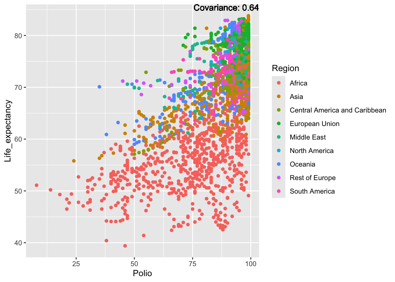

covariance_plot("Life_expectancy", "Diphtheria", df, sdf)

Warning in geom_text(aes(label = paste("Covariance:", round(cov(std_data_frame[[y_val]], : All aesthetics have length 1, but the data has 2864 rows.
ℹ Please consider using `annotate()` or provide this layer with data containing
  a single row.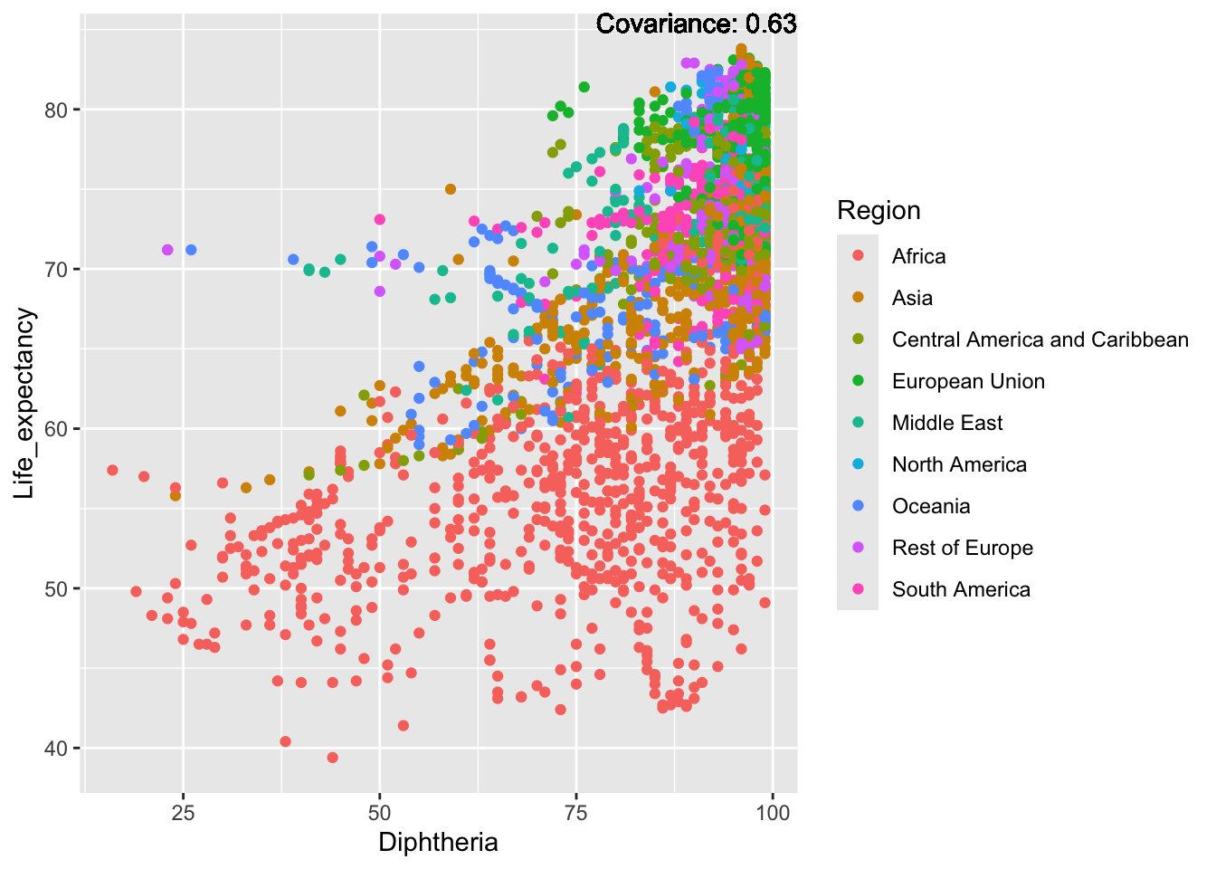

covariance_plot("Life_expectancy", "Incidents_HIV", df, sdf)

Warning in geom_text(aes(label = paste("Covariance:", round(cov(std_data_frame[[y_val]], : All aesthetics have length 1, but the data has 2864 rows.
ℹ Please consider using `annotate()` or provide this layer with data containing
  a single row.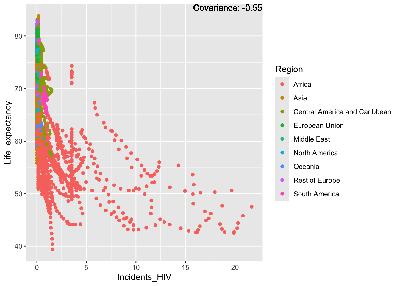

covariance_plot("Life_expectancy", "GDP_per_capita", df, sdf)

Warning in geom_text(aes(label = paste("Covariance:", round(cov(std_data_frame[[y_val]], : All aesthetics have length 1, but the data has 2864 rows.
ℹ Please consider using `annotate()` or provide this layer with data containing
  a single row.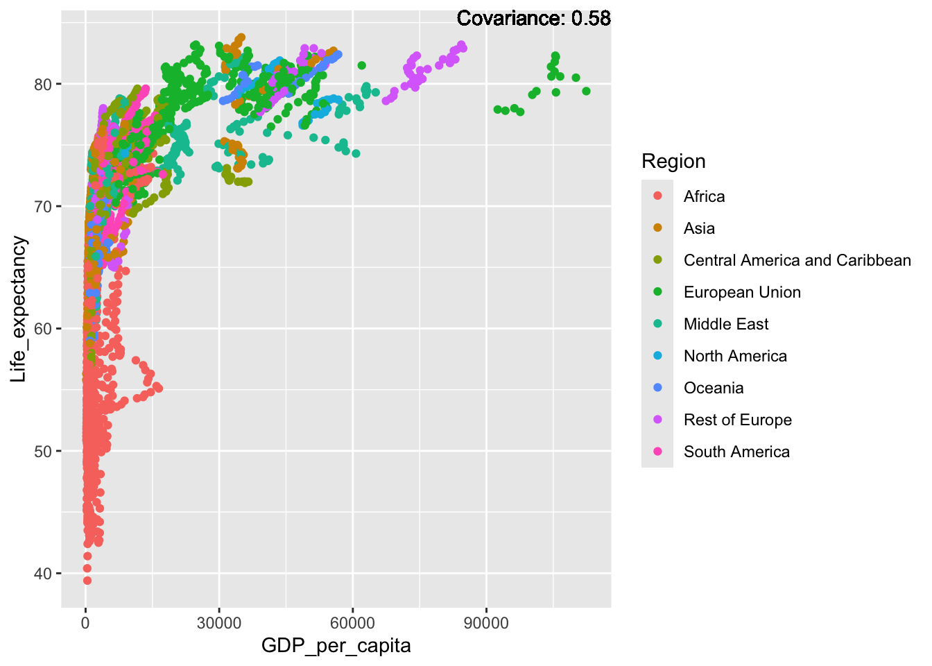

covariance_plot("Life_expectancy", "Population_mln", df, sdf)

Warning in geom_text(aes(label = paste("Covariance:", round(cov(std_data_frame[[y_val]], : All aesthetics have length 1, but the data has 2864 rows.
ℹ Please consider using `annotate()` or provide this layer with data containing
  a single row.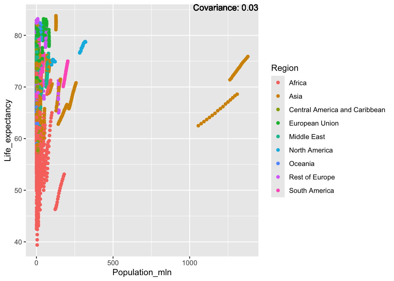

covariance_plot("Life_expectancy", "Thinness_ten_nineteen_years", df, sdf)

Warning in geom_text(aes(label = paste("Covariance:", round(cov(std_data_frame[[y_val]], : All aesthetics have length 1, but the data has 2864 rows.
ℹ Please consider using `annotate()` or provide this layer with data containing
  a single row.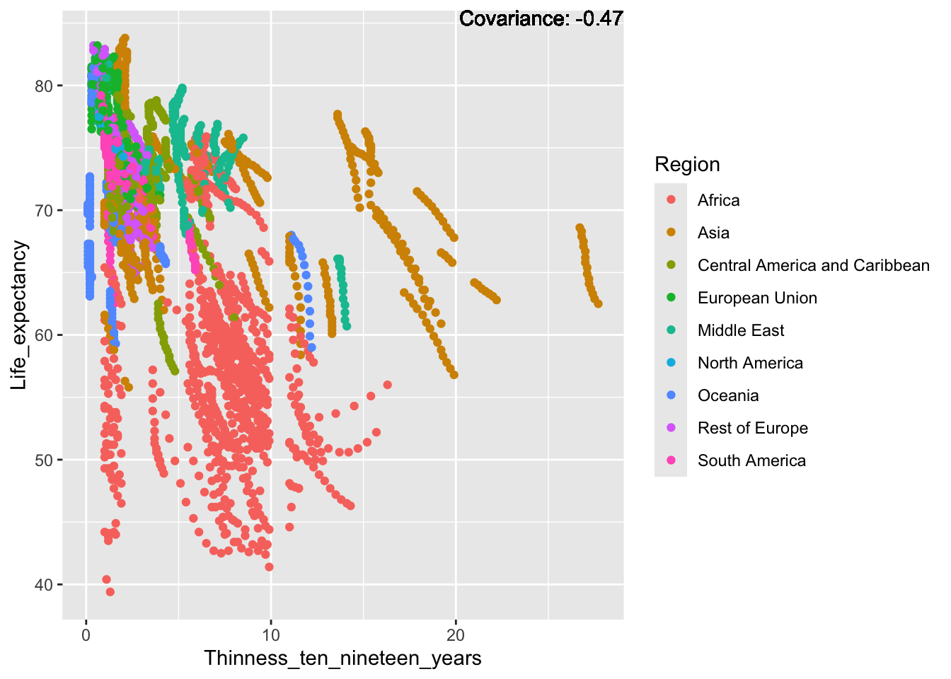

covariance_plot("Life_expectancy", "Thinness_five_nine_years", df, sdf)

Warning in geom_text(aes(label = paste("Covariance:", round(cov(std_data_frame[[y_val]], : All aesthetics have length 1, but the data has 2864 rows.
ℹ Please consider using `annotate()` or provide this layer with data containing
  a single row.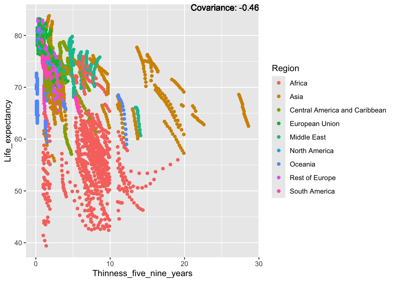

covariance_plot("Life_expectancy", "Schooling", df, sdf)

Warning in geom_text(aes(label = paste("Covariance:", round(cov(std_data_frame[[y_val]], : All aesthetics have length 1, but the data has 2864 rows.
ℹ Please consider using `annotate()` or provide this layer with data containing
  a single row.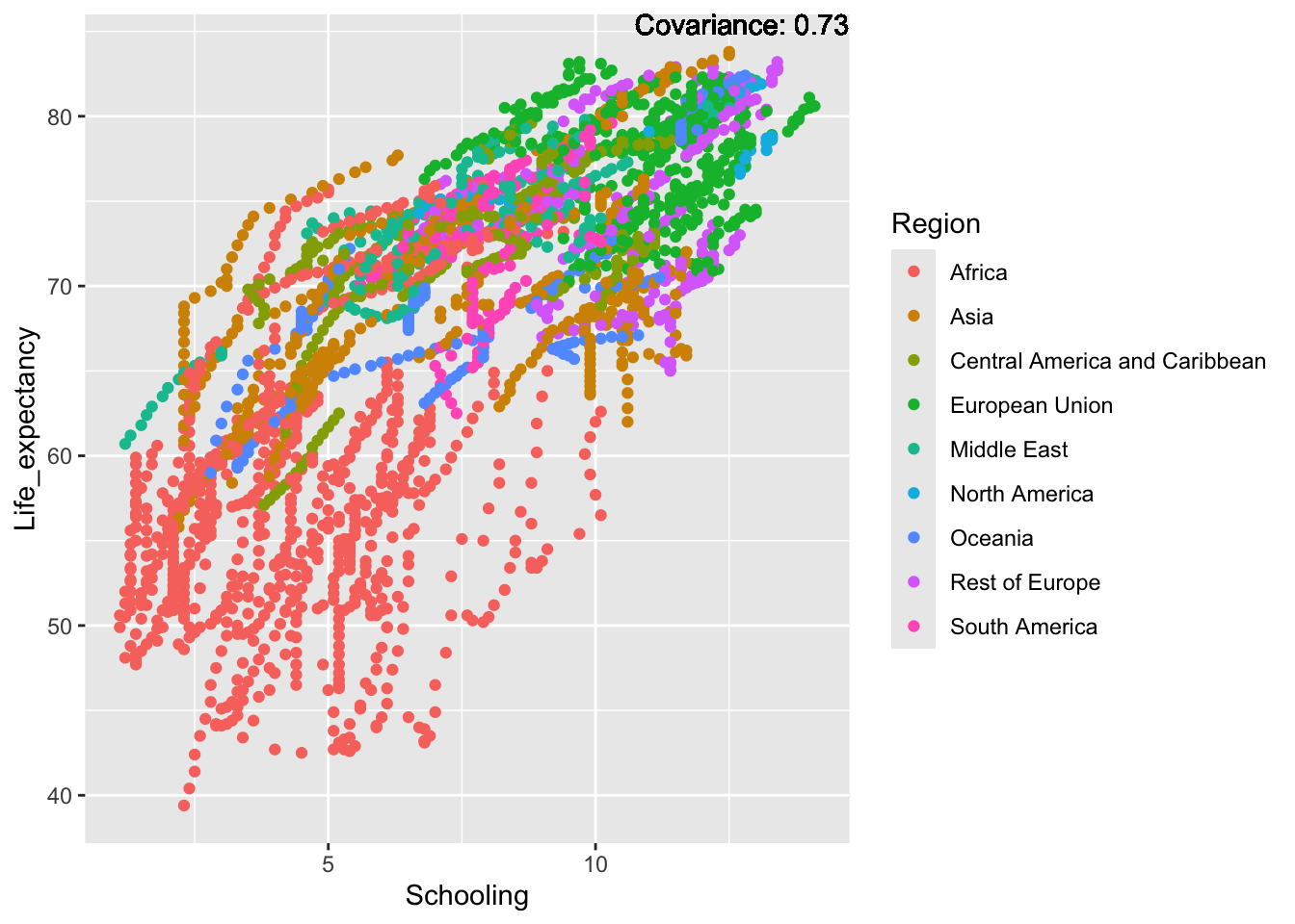

Inference:

Strong negative: adult mortality, infant deaths, under five deaths

Negative: HIV, thinness

Slight positive: Alcohol consumption, Hepatitis B, measles

Positive: BMI, Polio, Diphtheria, Schooling

Alcohol Consumption:

covariance_plot("Alcohol_consumption", "Adult_mortality", df, sdf)

Warning in geom_text(aes(label = paste("Covariance:", round(cov(std_data_frame[[y_val]], : All aesthetics have length 1, but the data has 2864 rows.
ℹ Please consider using `annotate()` or provide this layer with data containing
  a single row.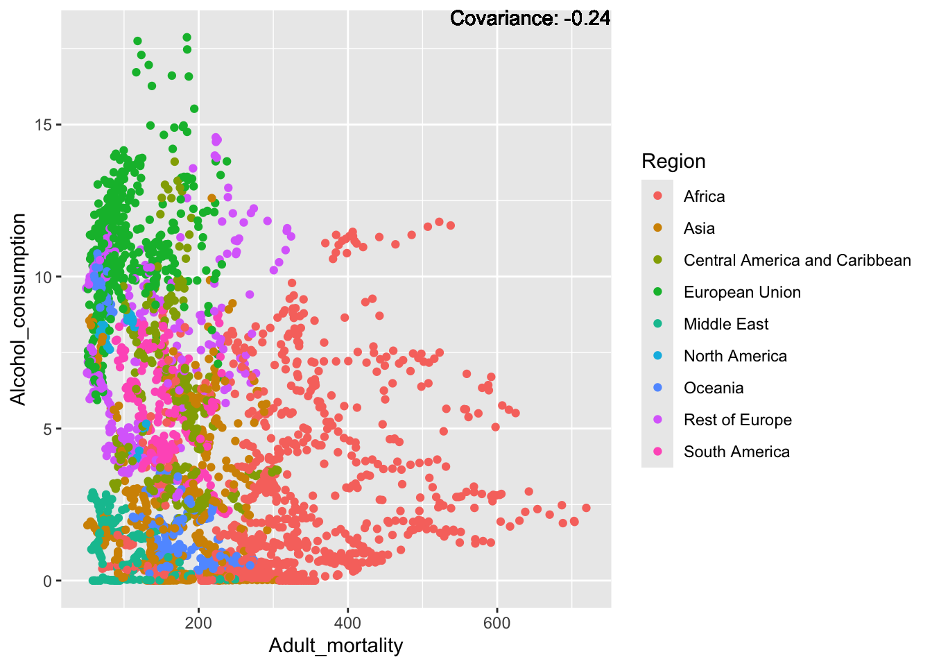

covariance_plot("Alcohol_consumption", "Infant_deaths", df, sdf)

Warning in geom_text(aes(label = paste("Covariance:", round(cov(std_data_frame[[y_val]], : All aesthetics have length 1, but the data has 2864 rows.
ℹ Please consider using `annotate()` or provide this layer with data containing
  a single row.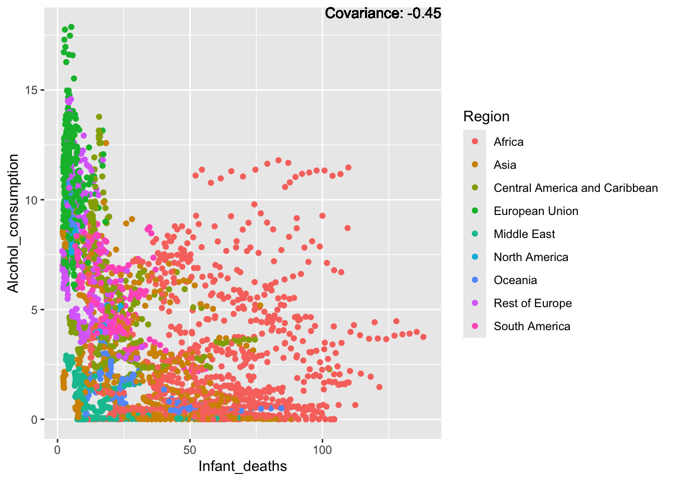

covariance_plot("Alcohol_consumption", "Under_five_deaths", df, sdf)

Warning in geom_text(aes(label = paste("Covariance:", round(cov(std_data_frame[[y_val]], : All aesthetics have length 1, but the data has 2864 rows.
ℹ Please consider using `annotate()` or provide this layer with data containing
  a single row.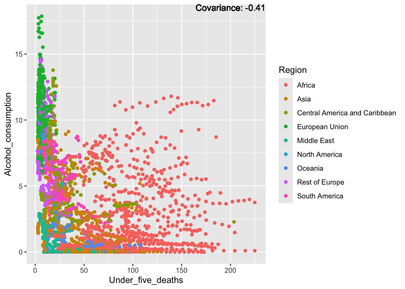

covariance_plot("Alcohol_consumption", "Life_expectancy", df, sdf)

Warning in geom_text(aes(label = paste("Covariance:", round(cov(std_data_frame[[y_val]], : All aesthetics have length 1, but the data has 2864 rows.
ℹ Please consider using `annotate()` or provide this layer with data containing
  a single row.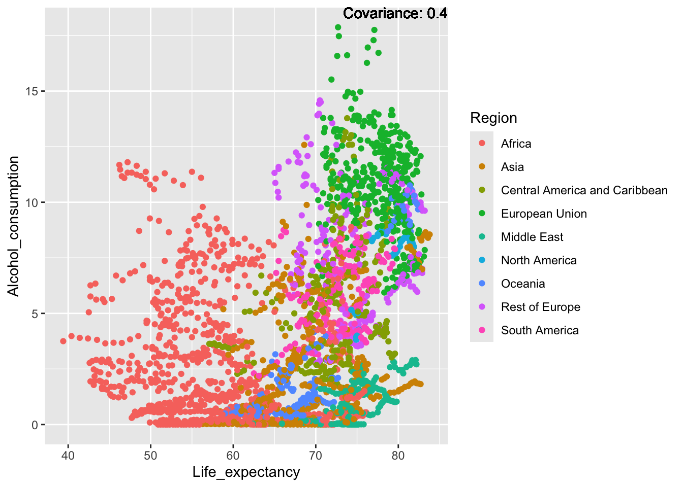

covariance_plot("Alcohol_consumption", "Hepatitis_B", df, sdf)

Warning in geom_text(aes(label = paste("Covariance:", round(cov(std_data_frame[[y_val]], : All aesthetics have length 1, but the data has 2864 rows.
ℹ Please consider using `annotate()` or provide this layer with data containing
  a single row.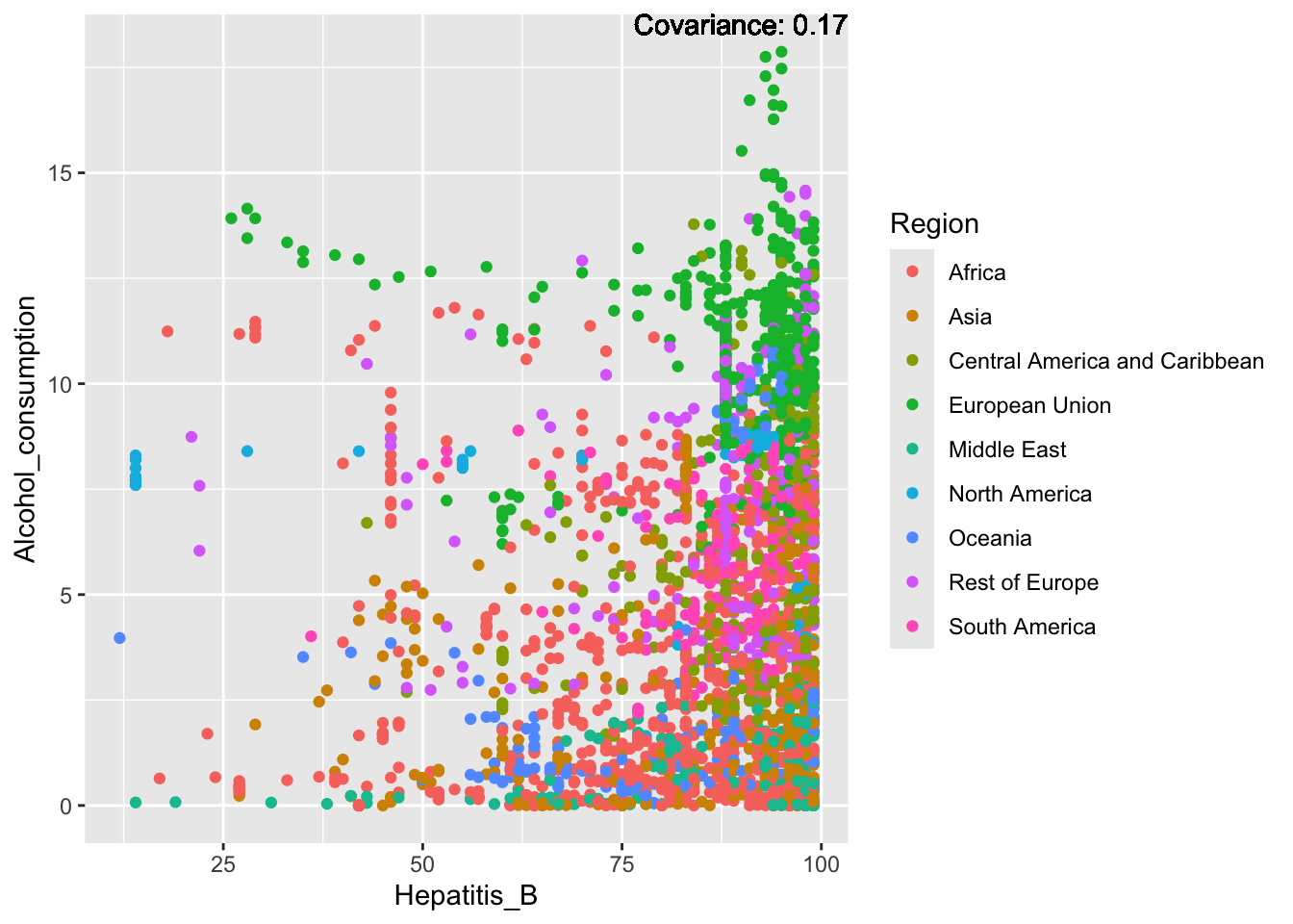

covariance_plot("Alcohol_consumption", "Measles", df, sdf)

Warning in geom_text(aes(label = paste("Covariance:", round(cov(std_data_frame[[y_val]], : All aesthetics have length 1, but the data has 2864 rows.
ℹ Please consider using `annotate()` or provide this layer with data containing
  a single row.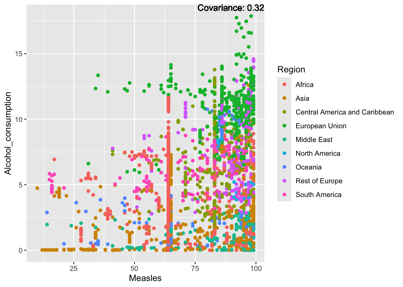

covariance_plot("Alcohol_consumption", "BMI", df, sdf)

Warning in geom_text(aes(label = paste("Covariance:", round(cov(std_data_frame[[y_val]], : All aesthetics have length 1, but the data has 2864 rows.
ℹ Please consider using `annotate()` or provide this layer with data containing
  a single row.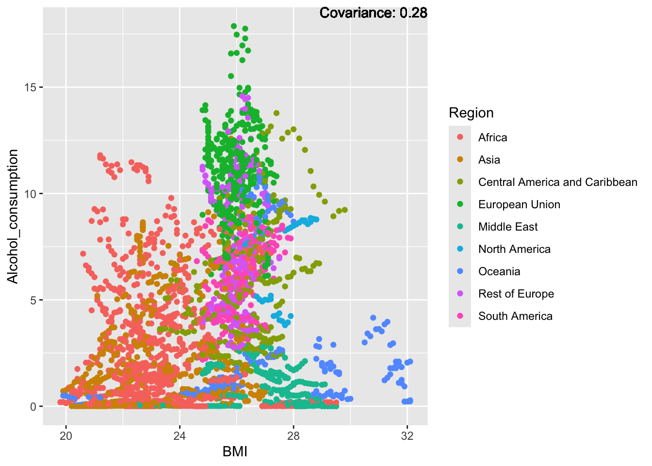

covariance_plot("Alcohol_consumption", "Polio", df, sdf)

Warning in geom_text(aes(label = paste("Covariance:", round(cov(std_data_frame[[y_val]], : All aesthetics have length 1, but the data has 2864 rows.
ℹ Please consider using `annotate()` or provide this layer with data containing
  a single row.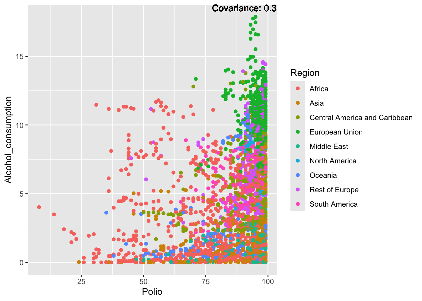

covariance_plot("Alcohol_consumption", "Diphtheria", df, sdf)

Warning in geom_text(aes(label = paste("Covariance:", round(cov(std_data_frame[[y_val]], : All aesthetics have length 1, but the data has 2864 rows.
ℹ Please consider using `annotate()` or provide this layer with data containing
  a single row.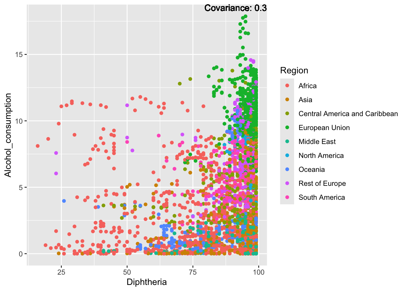

covariance_plot("Alcohol_consumption", "Incidents_HIV", df, sdf)

Warning in geom_text(aes(label = paste("Covariance:", round(cov(std_data_frame[[y_val]], : All aesthetics have length 1, but the data has 2864 rows.
ℹ Please consider using `annotate()` or provide this layer with data containing
  a single row.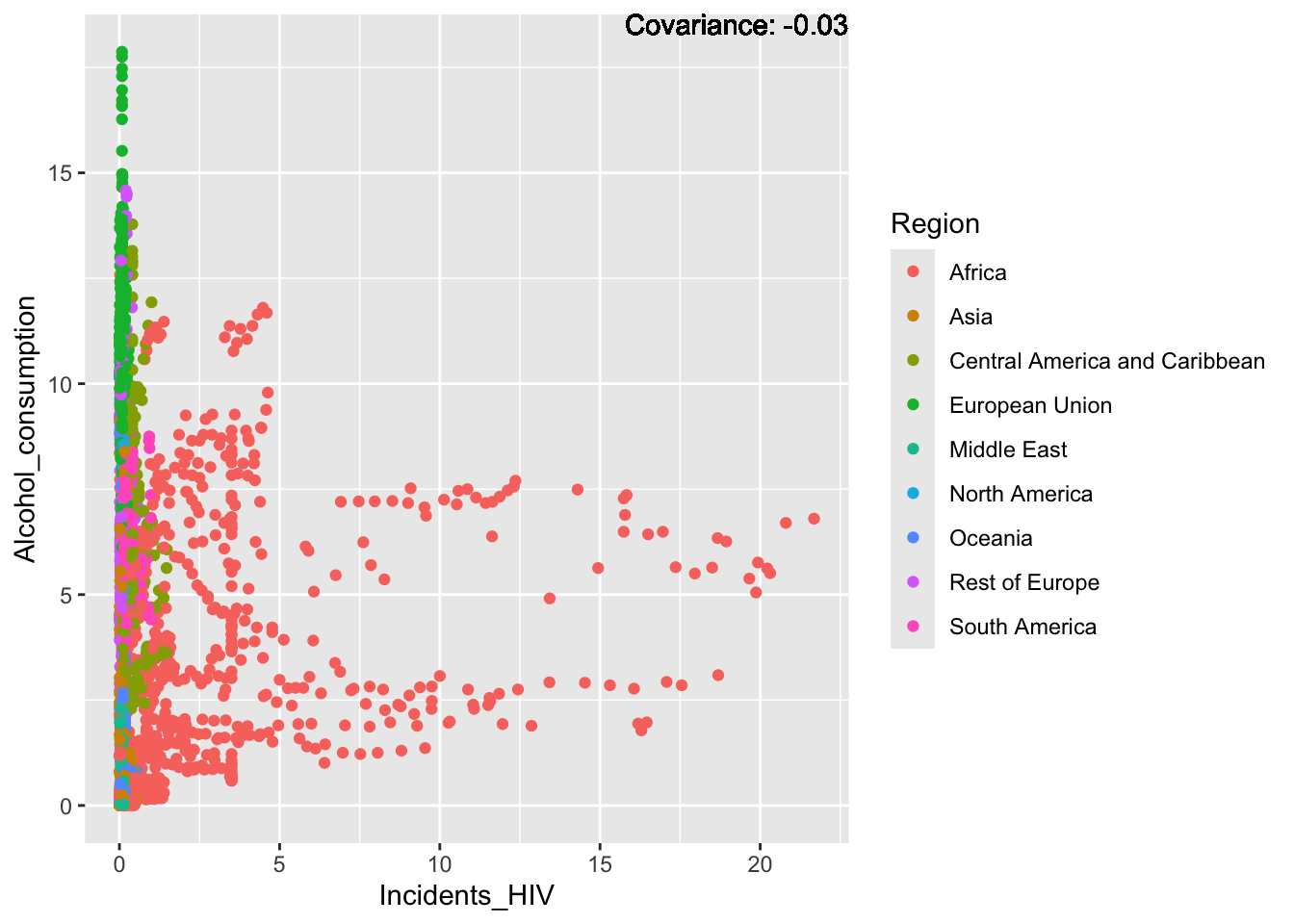

covariance_plot("Alcohol_consumption", "GDP_per_capita", df, sdf)

Warning in geom_text(aes(label = paste("Covariance:", round(cov(std_data_frame[[y_val]], : All aesthetics have length 1, but the data has 2864 rows.
ℹ Please consider using `annotate()` or provide this layer with data containing
  a single row.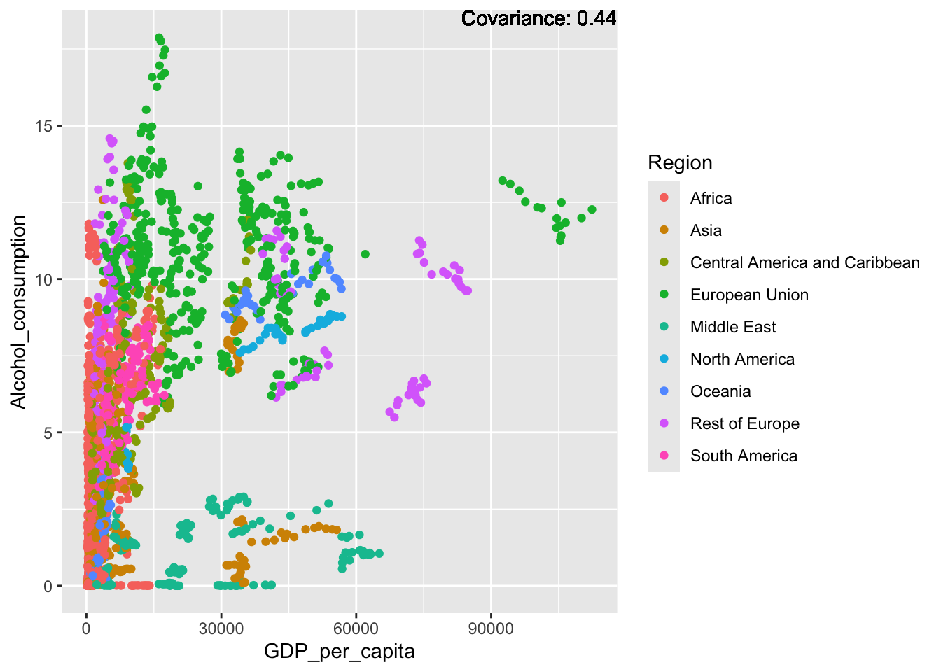

covariance_plot("Alcohol_consumption", "Population_mln", df, sdf)

Warning in geom_text(aes(label = paste("Covariance:", round(cov(std_data_frame[[y_val]], : All aesthetics have length 1, but the data has 2864 rows.
ℹ Please consider using `annotate()` or provide this layer with data containing
  a single row.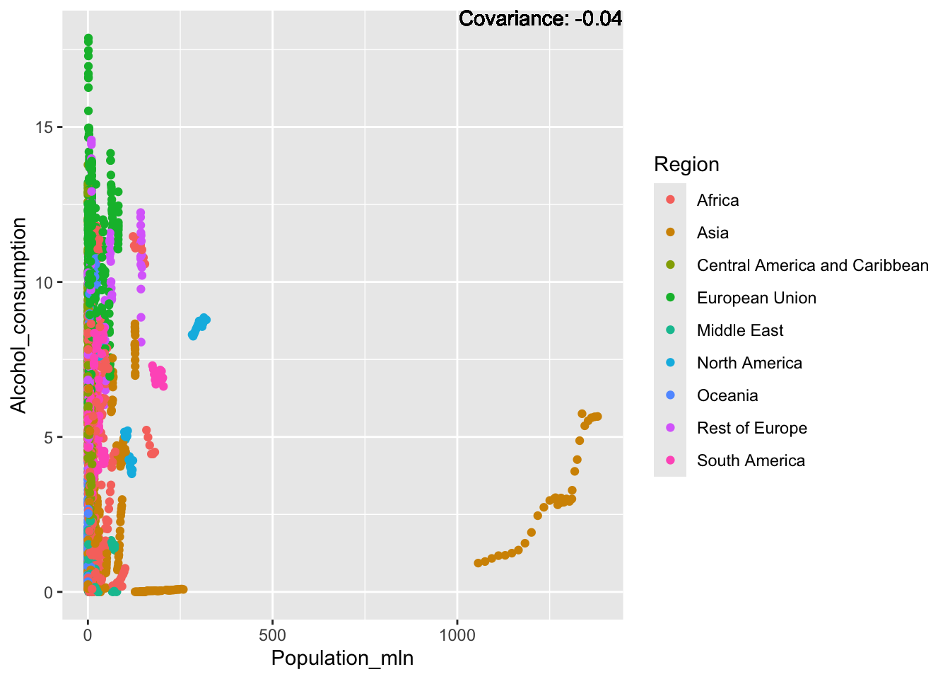

covariance_plot("Alcohol_consumption", "Thinness_ten_nineteen_years", df, sdf)

Warning in geom_text(aes(label = paste("Covariance:", round(cov(std_data_frame[[y_val]], : All aesthetics have length 1, but the data has 2864 rows.
ℹ Please consider using `annotate()` or provide this layer with data containing
  a single row.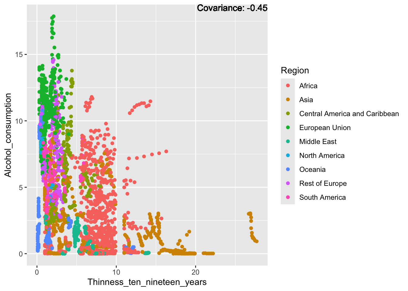

covariance_plot("Alcohol_consumption", "Thinness_five_nine_years", df, sdf)

Warning in geom_text(aes(label = paste("Covariance:", round(cov(std_data_frame[[y_val]], : All aesthetics have length 1, but the data has 2864 rows.
ℹ Please consider using `annotate()` or provide this layer with data containing
  a single row.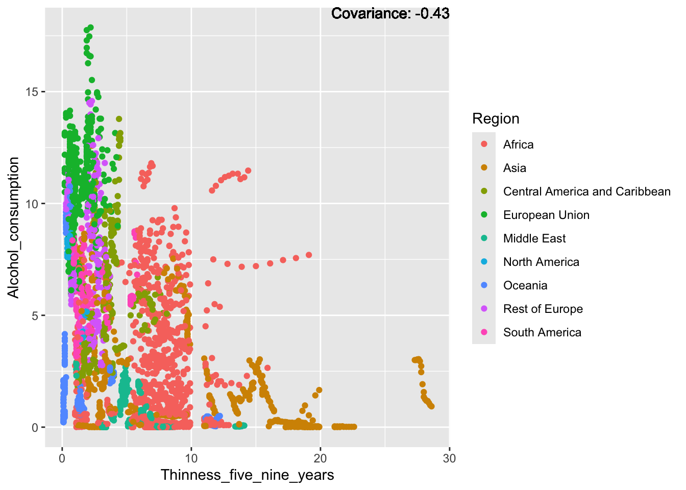

covariance_plot("Alcohol_consumption", "Schooling", df, sdf)

Warning in geom_text(aes(label = paste("Covariance:", round(cov(std_data_frame[[y_val]], : All aesthetics have length 1, but the data has 2864 rows.
ℹ Please consider using `annotate()` or provide this layer with data containing
  a single row.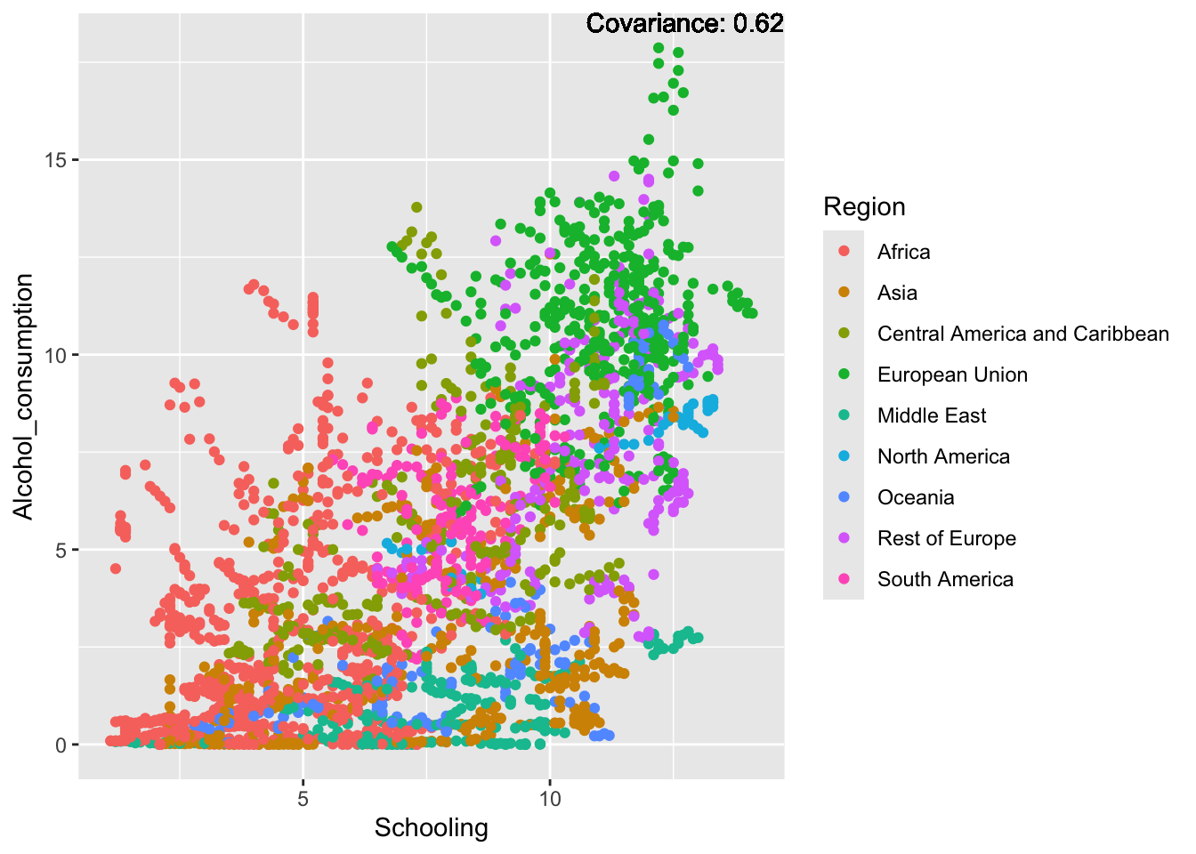

Inferences:

There is a positive relationship between Schooling and alcohol consumption,

Some positive relationship: GDP

Some negative relationship: Infant deaths

Strong negative relationship: Population

Other variables have some covariance, but it does not seem to be strongly related.

GDP:

covariance_plot("GDP_per_capita", "Adult_mortality", df, sdf)

Warning in geom_text(aes(label = paste("Covariance:", round(cov(std_data_frame[[y_val]], : All aesthetics have length 1, but the data has 2864 rows.
ℹ Please consider using `annotate()` or provide this layer with data containing
  a single row.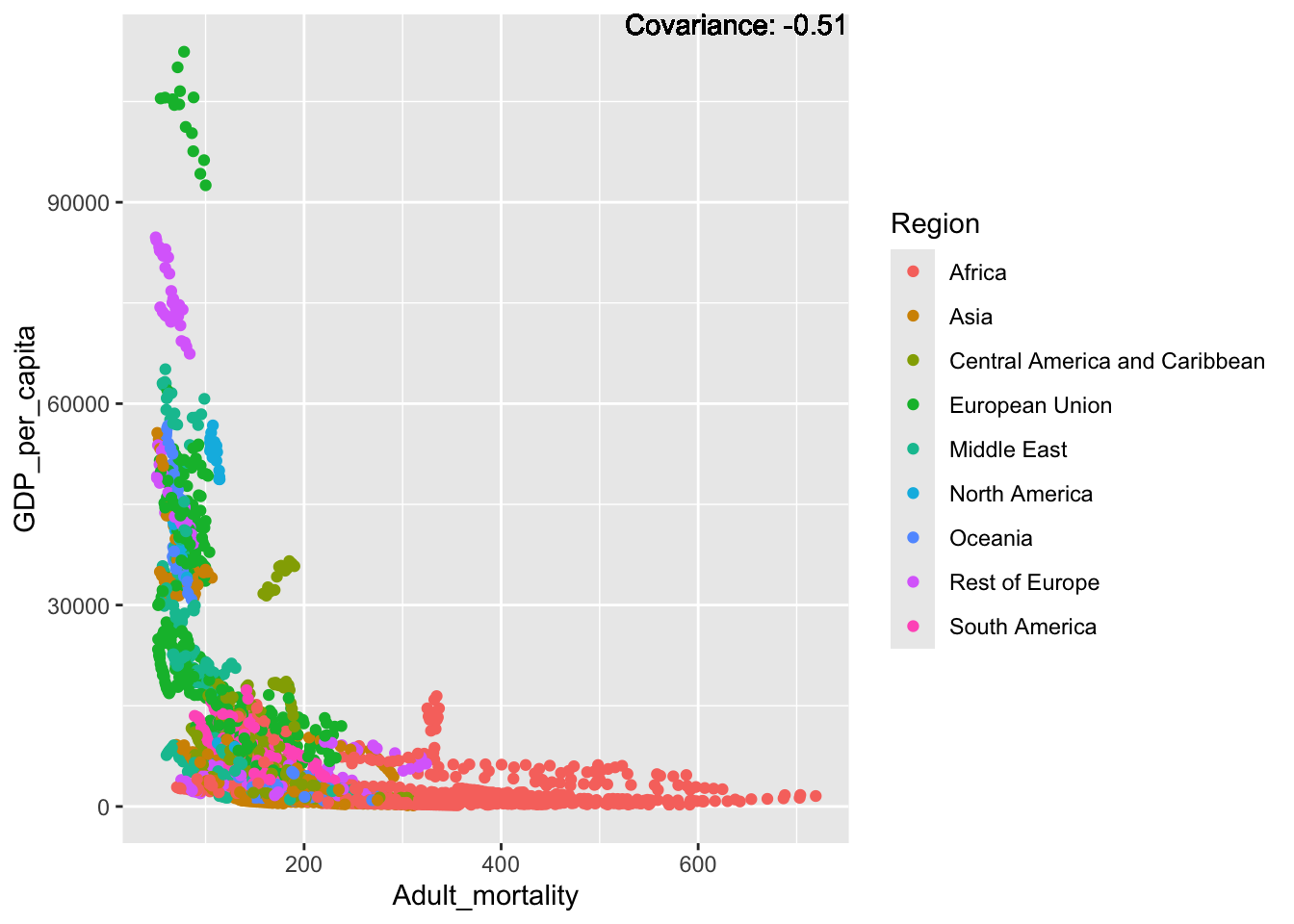

covariance_plot("GDP_per_capita", "Infant_deaths", df, sdf)

Warning in geom_text(aes(label = paste("Covariance:", round(cov(std_data_frame[[y_val]], : All aesthetics have length 1, but the data has 2864 rows.
ℹ Please consider using `annotate()` or provide this layer with data containing
  a single row.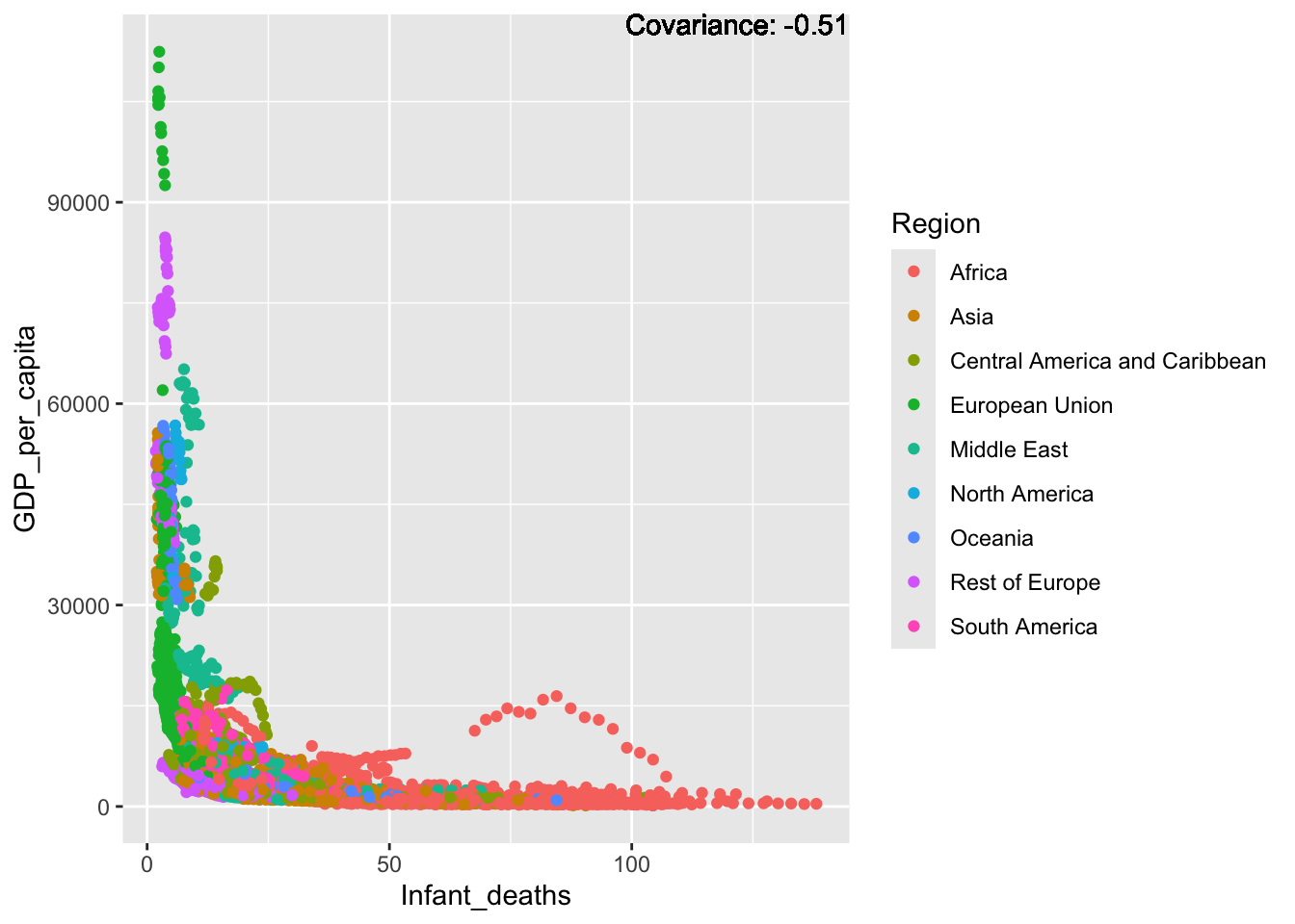

covariance_plot("GDP_per_capita", "Under_five_deaths", df, sdf)

Warning in geom_text(aes(label = paste("Covariance:", round(cov(std_data_frame[[y_val]], : All aesthetics have length 1, but the data has 2864 rows.
ℹ Please consider using `annotate()` or provide this layer with data containing
  a single row.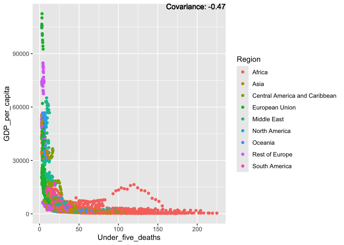

covariance_plot("GDP_per_capita", "Life_expectancy", df, sdf)

Warning in geom_text(aes(label = paste("Covariance:", round(cov(std_data_frame[[y_val]], : All aesthetics have length 1, but the data has 2864 rows.
ℹ Please consider using `annotate()` or provide this layer with data containing
  a single row.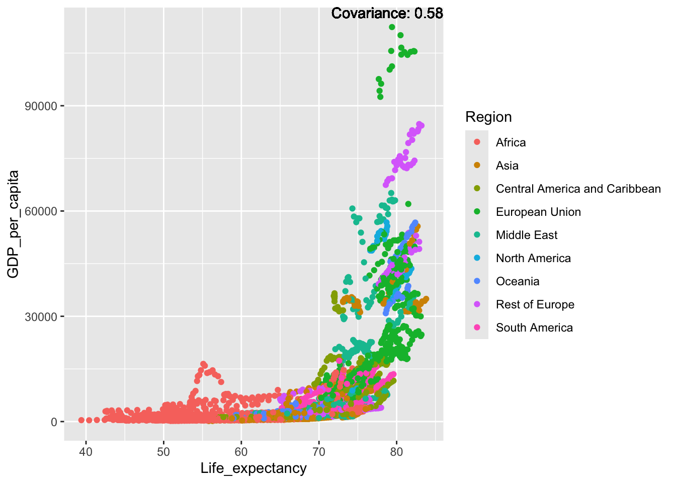

covariance_plot("GDP_per_capita", "Hepatitis_B", df, sdf)

Warning in geom_text(aes(label = paste("Covariance:", round(cov(std_data_frame[[y_val]], : All aesthetics have length 1, but the data has 2864 rows.
ℹ Please consider using `annotate()` or provide this layer with data containing
  a single row.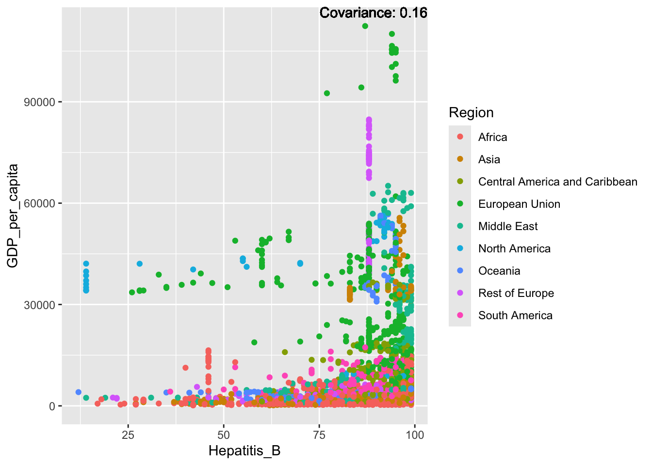

covariance_plot("GDP_per_capita", "Measles", df, sdf)

Warning in geom_text(aes(label = paste("Covariance:", round(cov(std_data_frame[[y_val]], : All aesthetics have length 1, but the data has 2864 rows.
ℹ Please consider using `annotate()` or provide this layer with data containing
  a single row.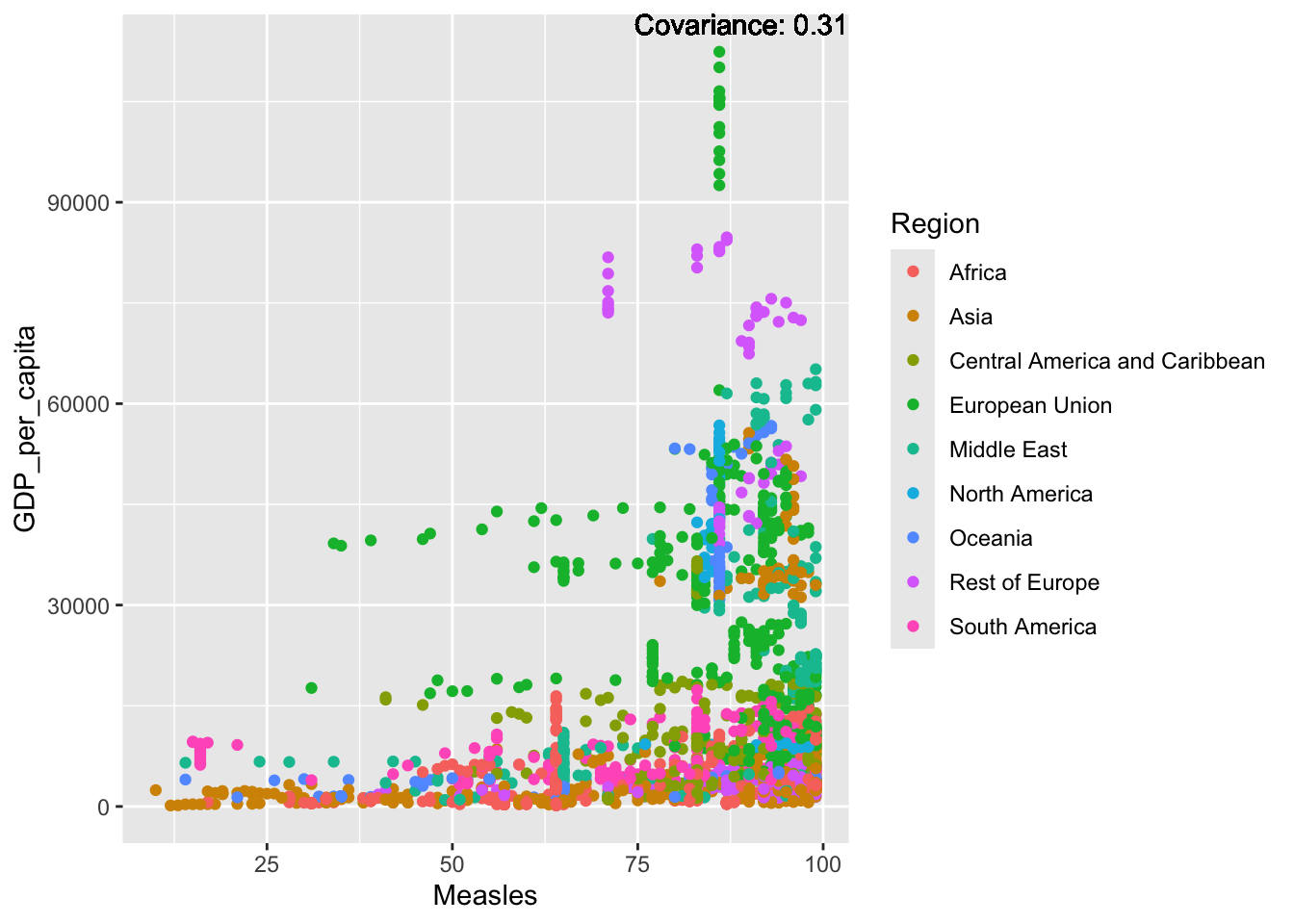

covariance_plot("GDP_per_capita", "BMI", df, sdf)

Warning in geom_text(aes(label = paste("Covariance:", round(cov(std_data_frame[[y_val]], : All aesthetics have length 1, but the data has 2864 rows.
ℹ Please consider using `annotate()` or provide this layer with data containing
  a single row.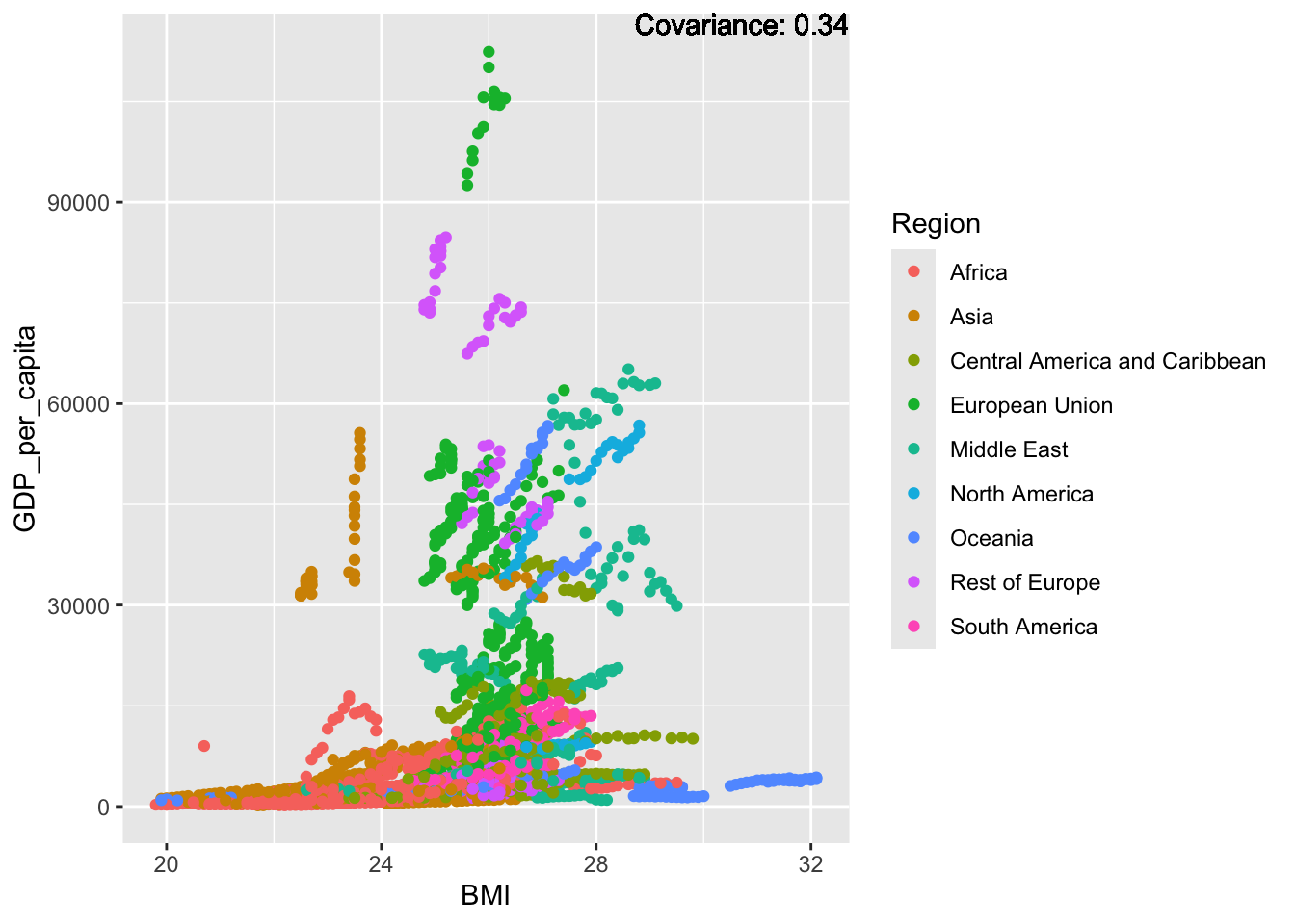

covariance_plot("GDP_per_capita", "Polio", df, sdf)

Warning in geom_text(aes(label = paste("Covariance:", round(cov(std_data_frame[[y_val]], : All aesthetics have length 1, but the data has 2864 rows.
ℹ Please consider using `annotate()` or provide this layer with data containing
  a single row.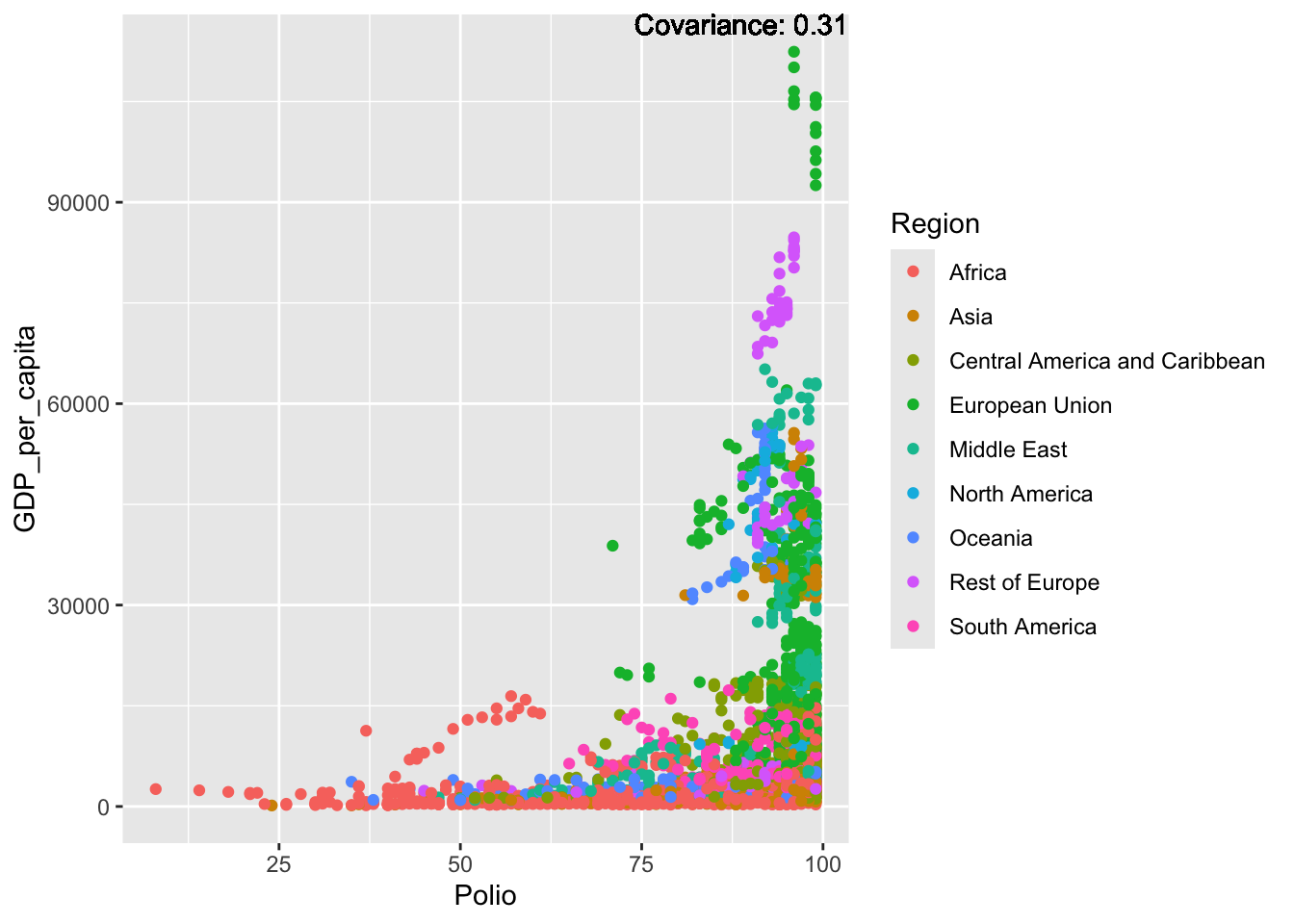

covariance_plot("GDP_per_capita", "Diphtheria", df, sdf)

Warning in geom_text(aes(label = paste("Covariance:", round(cov(std_data_frame[[y_val]], : All aesthetics have length 1, but the data has 2864 rows.
ℹ Please consider using `annotate()` or provide this layer with data containing
  a single row.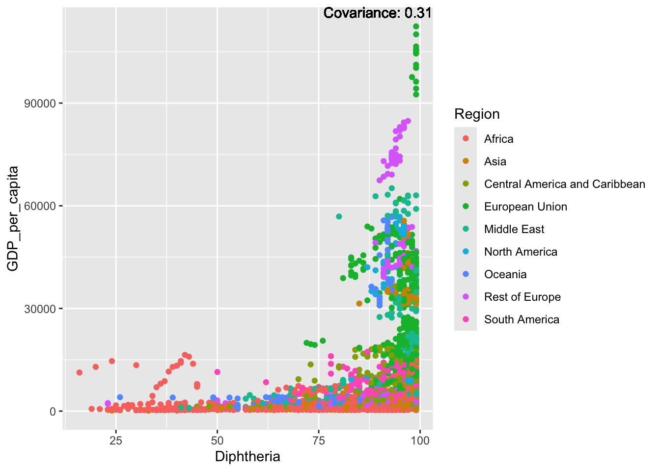

covariance_plot("GDP_per_capita", "Incidents_HIV", df, sdf)

Warning in geom_text(aes(label = paste("Covariance:", round(cov(std_data_frame[[y_val]], : All aesthetics have length 1, but the data has 2864 rows.
ℹ Please consider using `annotate()` or provide this layer with data containing
  a single row.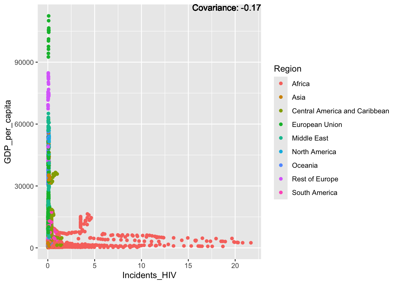

covariance_plot("GDP_per_capita", "Alcohol_consumption", df, sdf)

Warning in geom_text(aes(label = paste("Covariance:", round(cov(std_data_frame[[y_val]], : All aesthetics have length 1, but the data has 2864 rows.
ℹ Please consider using `annotate()` or provide this layer with data containing
  a single row.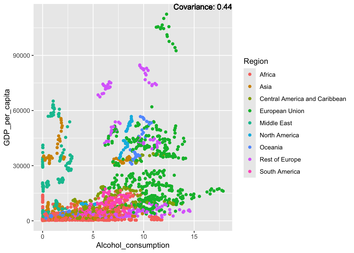

covariance_plot("GDP_per_capita", "Population_mln", df, sdf)

Warning in geom_text(aes(label = paste("Covariance:", round(cov(std_data_frame[[y_val]], : All aesthetics have length 1, but the data has 2864 rows.
ℹ Please consider using `annotate()` or provide this layer with data containing
  a single row.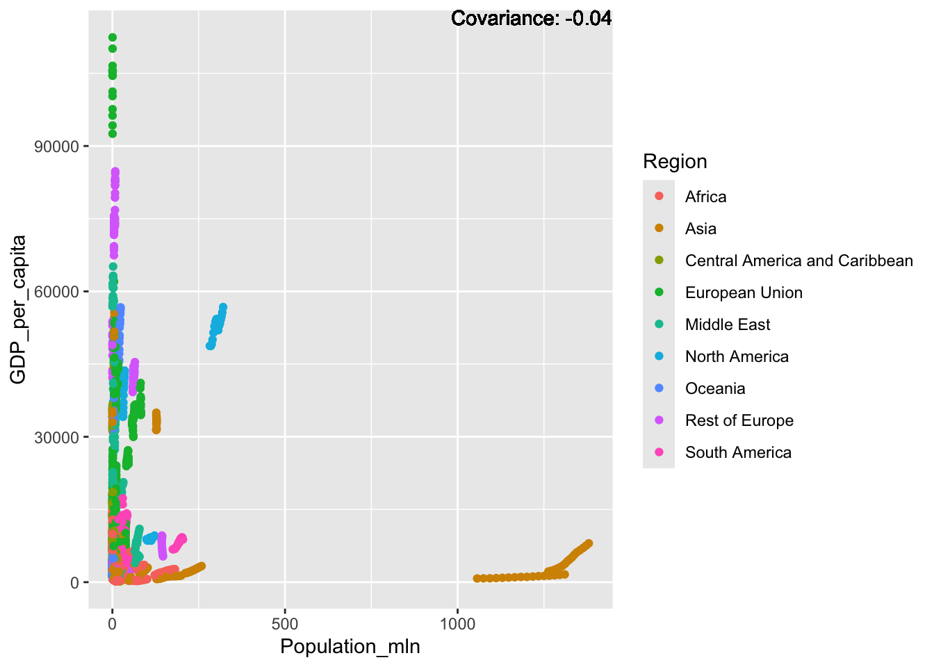

covariance_plot("GDP_per_capita", "Thinness_ten_nineteen_years", df, sdf)

Warning in geom_text(aes(label = paste("Covariance:", round(cov(std_data_frame[[y_val]], : All aesthetics have length 1, but the data has 2864 rows.
ℹ Please consider using `annotate()` or provide this layer with data containing
  a single row.

covariance_plot("GDP_per_capita", "Thinness_five_nine_years", df, sdf)

Warning in geom_text(aes(label = paste("Covariance:", round(cov(std_data_frame[[y_val]], : All aesthetics have length 1, but the data has 2864 rows.
ℹ Please consider using `annotate()` or provide this layer with data containing
  a single row.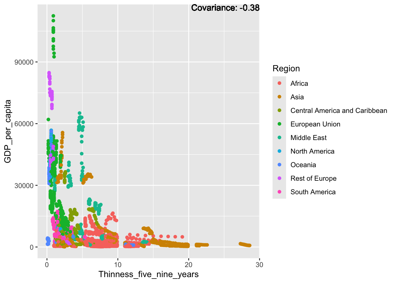

covariance_plot("GDP_per_capita", "Schooling", df, sdf)

Warning in geom_text(aes(label = paste("Covariance:", round(cov(std_data_frame[[y_val]], : All aesthetics have length 1, but the data has 2864 rows.
ℹ Please consider using `annotate()` or provide this layer with data containing
  a single row.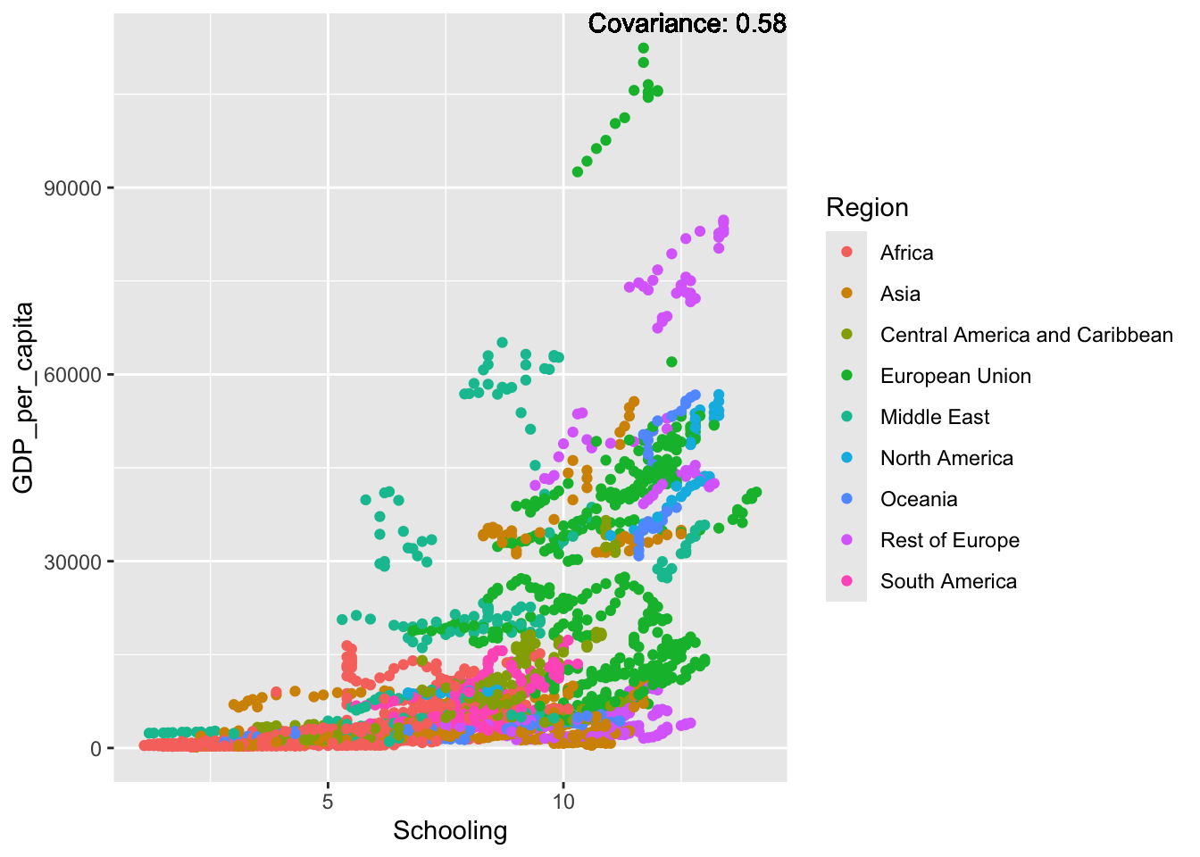

Inference:

Some positive relationship: Life expectancy, alcohol consumption, schooling

Some negative relationship: Infant deaths, under five deaths, adult mortality

Adult Mortality:

covariance_plot("Adult_mortality", "GDP_per_capita", df, sdf)

Warning in geom_text(aes(label = paste("Covariance:", round(cov(std_data_frame[[y_val]], : All aesthetics have length 1, but the data has 2864 rows.
ℹ Please consider using `annotate()` or provide this layer with data containing
  a single row.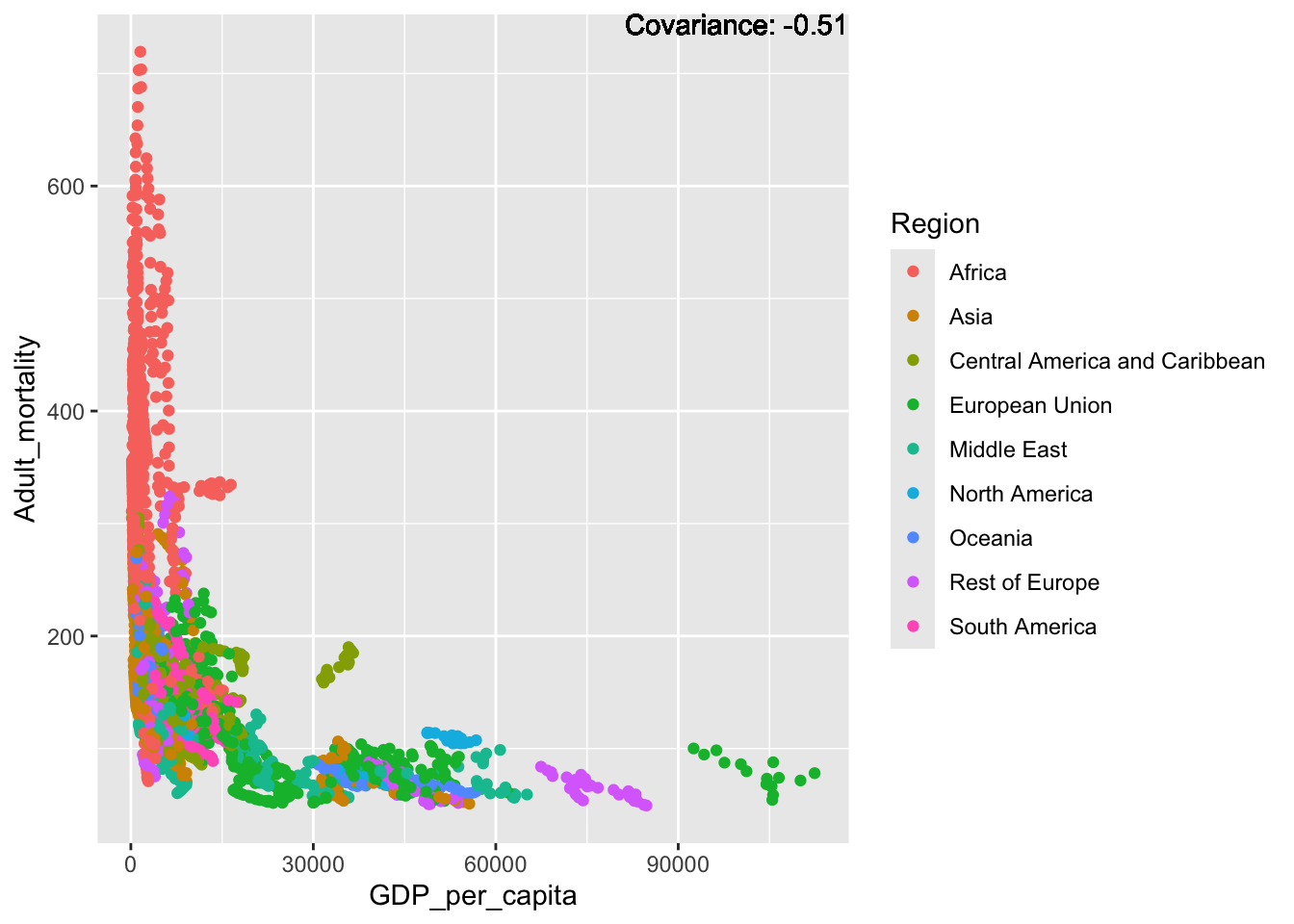

covariance_plot("Adult_mortality", "Infant_deaths", df, sdf)

Warning in geom_text(aes(label = paste("Covariance:", round(cov(std_data_frame[[y_val]], : All aesthetics have length 1, but the data has 2864 rows.
ℹ Please consider using `annotate()` or provide this layer with data containing
  a single row.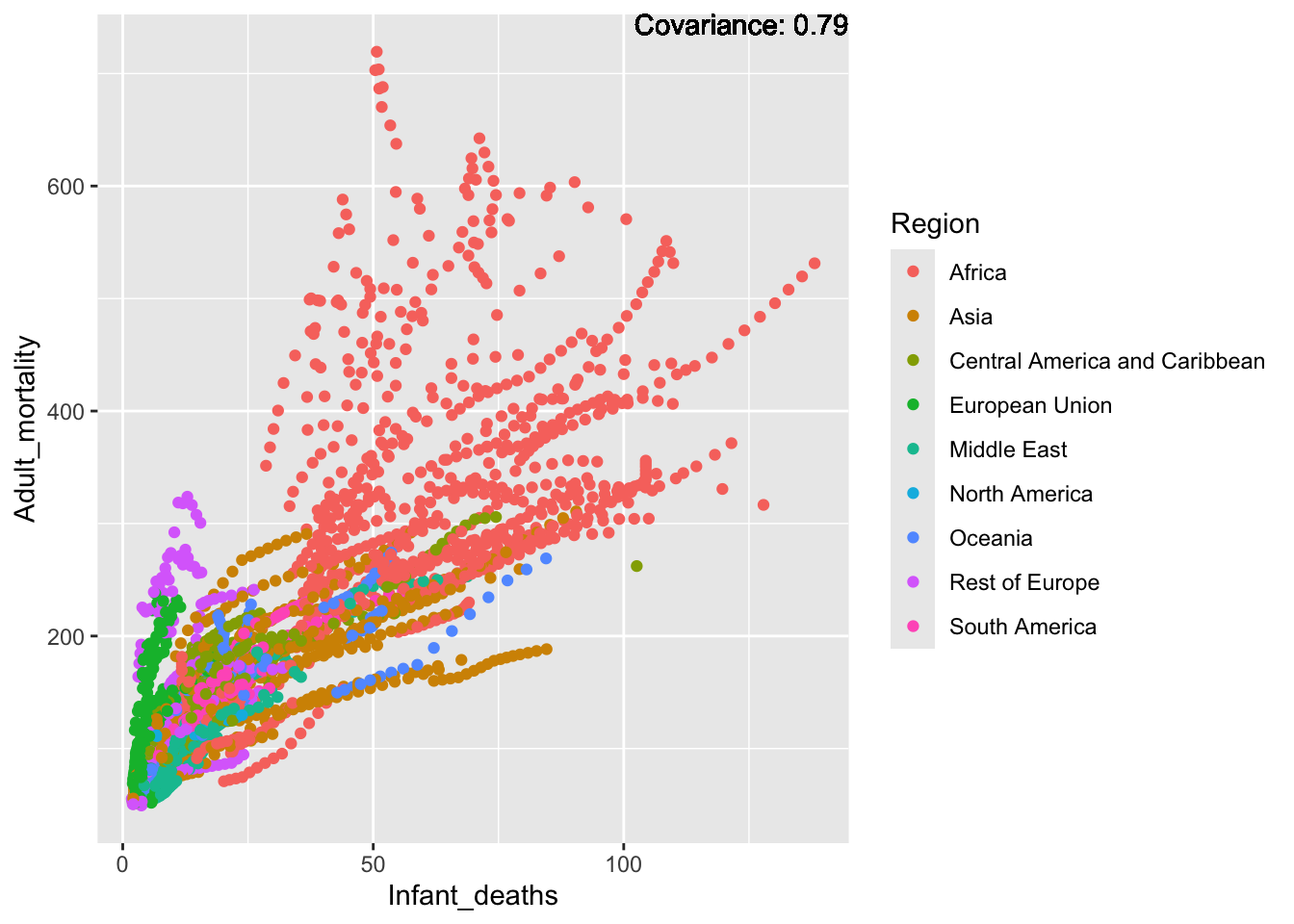

covariance_plot("Adult_mortality", "Under_five_deaths", df, sdf)

Warning in geom_text(aes(label = paste("Covariance:", round(cov(std_data_frame[[y_val]], : All aesthetics have length 1, but the data has 2864 rows.
ℹ Please consider using `annotate()` or provide this layer with data containing
  a single row.

covariance_plot("Adult_mortality", "Life_expectancy", df, sdf)

Warning in geom_text(aes(label = paste("Covariance:", round(cov(std_data_frame[[y_val]], : All aesthetics have length 1, but the data has 2864 rows.
ℹ Please consider using `annotate()` or provide this layer with data containing
  a single row.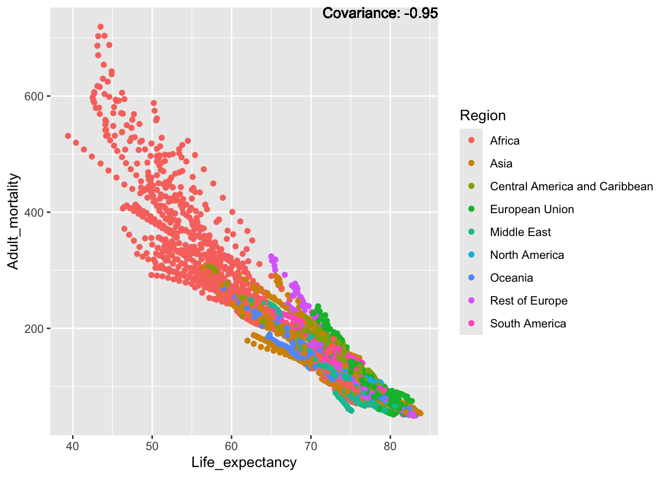

covariance_plot("Adult_mortality", "Hepatitis_B", df, sdf)

Warning in geom_text(aes(label = paste("Covariance:", round(cov(std_data_frame[[y_val]], : All aesthetics have length 1, but the data has 2864 rows.
ℹ Please consider using `annotate()` or provide this layer with data containing
  a single row.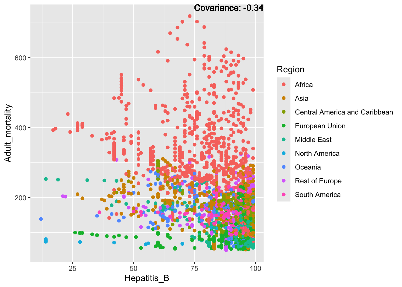

covariance_plot("Adult_mortality", "Measles", df, sdf)

Warning in geom_text(aes(label = paste("Covariance:", round(cov(std_data_frame[[y_val]], : All aesthetics have length 1, but the data has 2864 rows.
ℹ Please consider using `annotate()` or provide this layer with data containing
  a single row.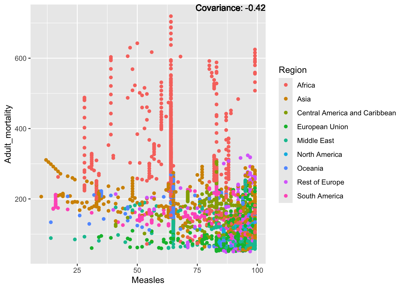

covariance_plot("Adult_mortality", "BMI", df, sdf)

Warning in geom_text(aes(label = paste("Covariance:", round(cov(std_data_frame[[y_val]], : All aesthetics have length 1, but the data has 2864 rows.
ℹ Please consider using `annotate()` or provide this layer with data containing
  a single row.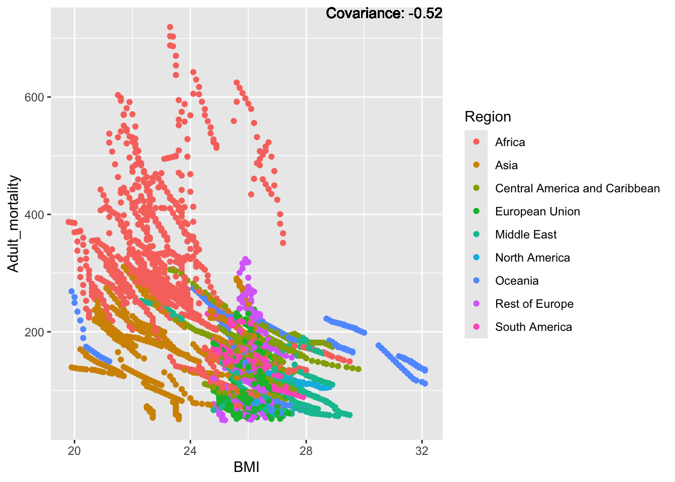

covariance_plot("Adult_mortality", "Polio", df, sdf)

Warning in geom_text(aes(label = paste("Covariance:", round(cov(std_data_frame[[y_val]], : All aesthetics have length 1, but the data has 2864 rows.
ℹ Please consider using `annotate()` or provide this layer with data containing
  a single row.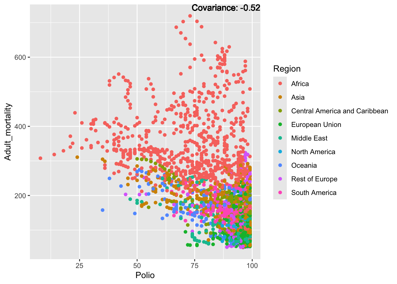

covariance_plot("Adult_mortality", "Diphtheria", df, sdf)

Warning in geom_text(aes(label = paste("Covariance:", round(cov(std_data_frame[[y_val]], : All aesthetics have length 1, but the data has 2864 rows.
ℹ Please consider using `annotate()` or provide this layer with data containing
  a single row.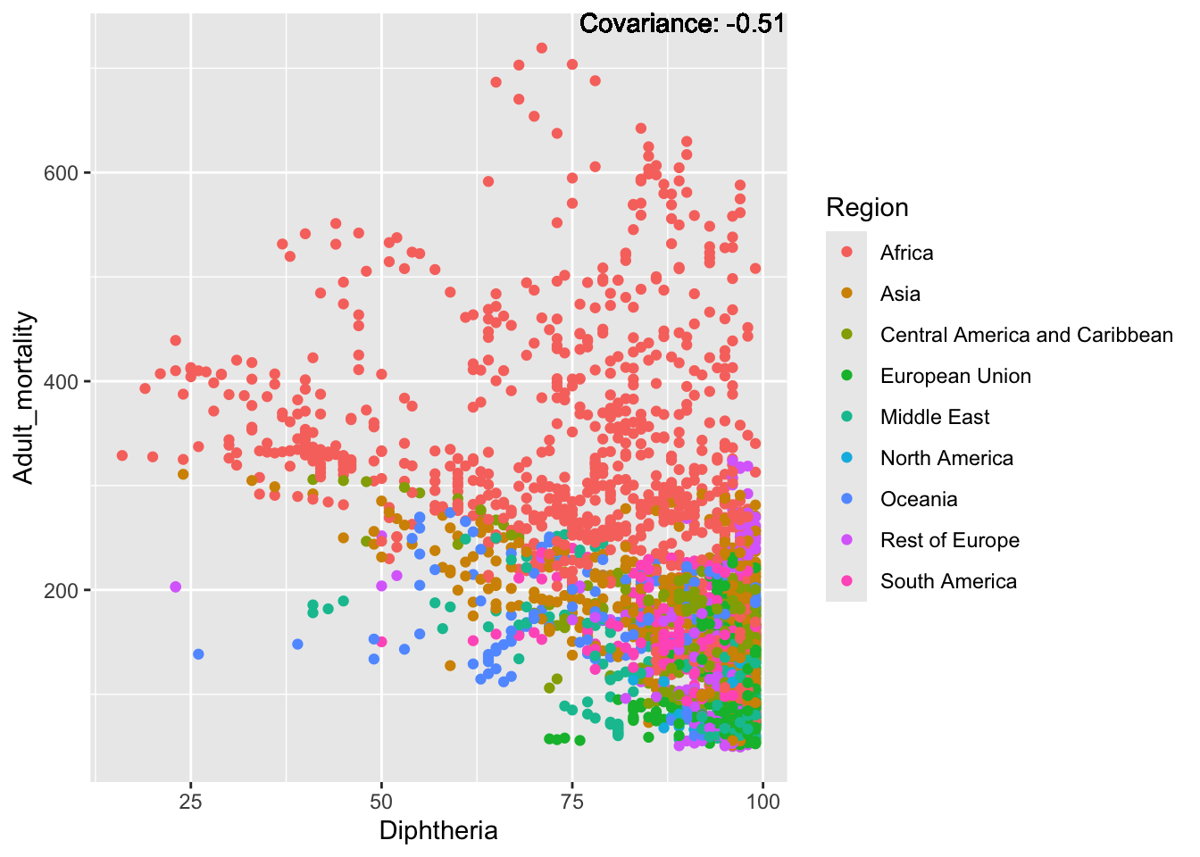

covariance_plot("Adult_mortality", "Incidents_HIV", df, sdf)

Warning in geom_text(aes(label = paste("Covariance:", round(cov(std_data_frame[[y_val]], : All aesthetics have length 1, but the data has 2864 rows.
ℹ Please consider using `annotate()` or provide this layer with data containing
  a single row.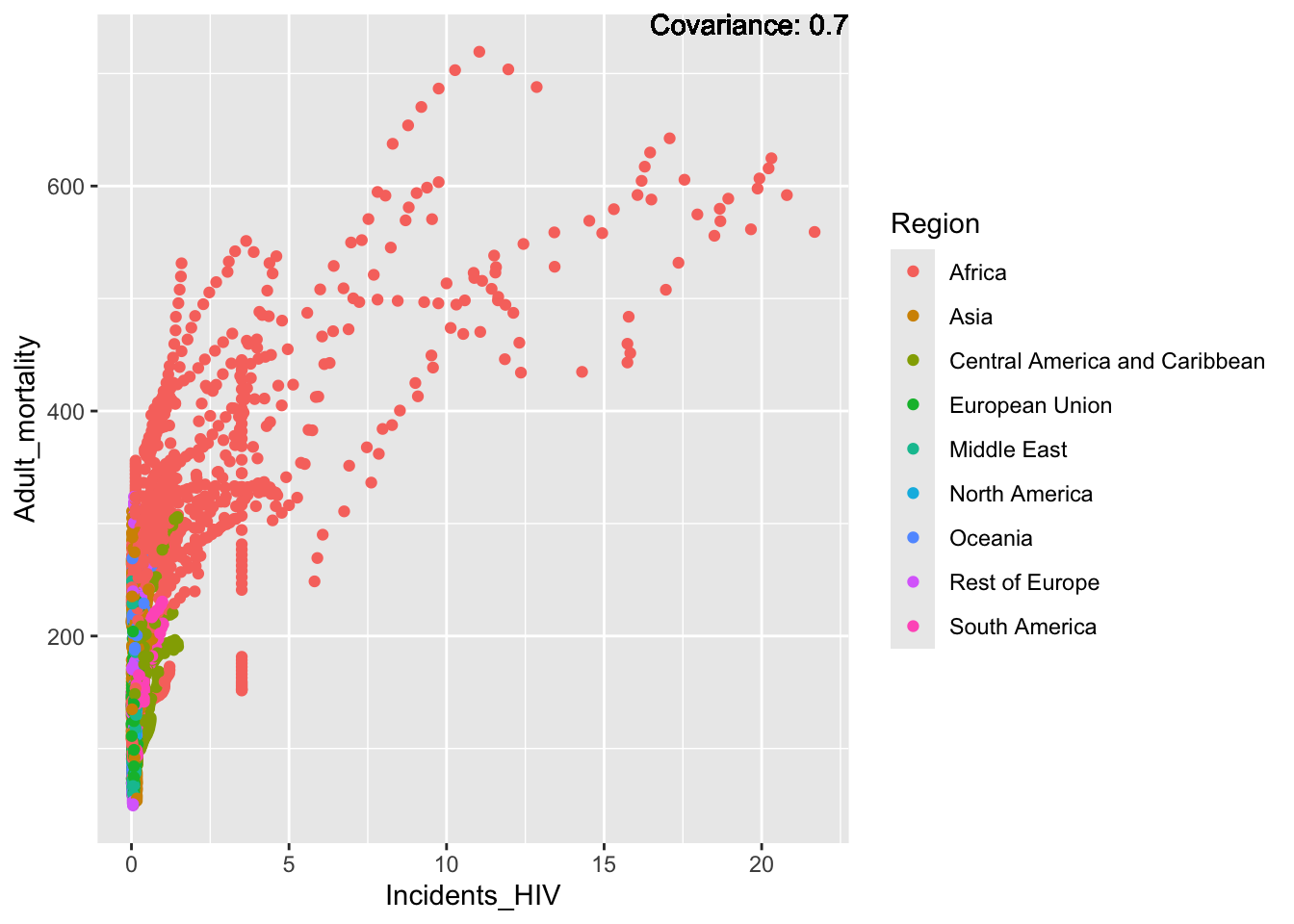

covariance_plot("Adult_mortality", "Alcohol_consumption", df, sdf)

Warning in geom_text(aes(label = paste("Covariance:", round(cov(std_data_frame[[y_val]], : All aesthetics have length 1, but the data has 2864 rows.
ℹ Please consider using `annotate()` or provide this layer with data containing
  a single row.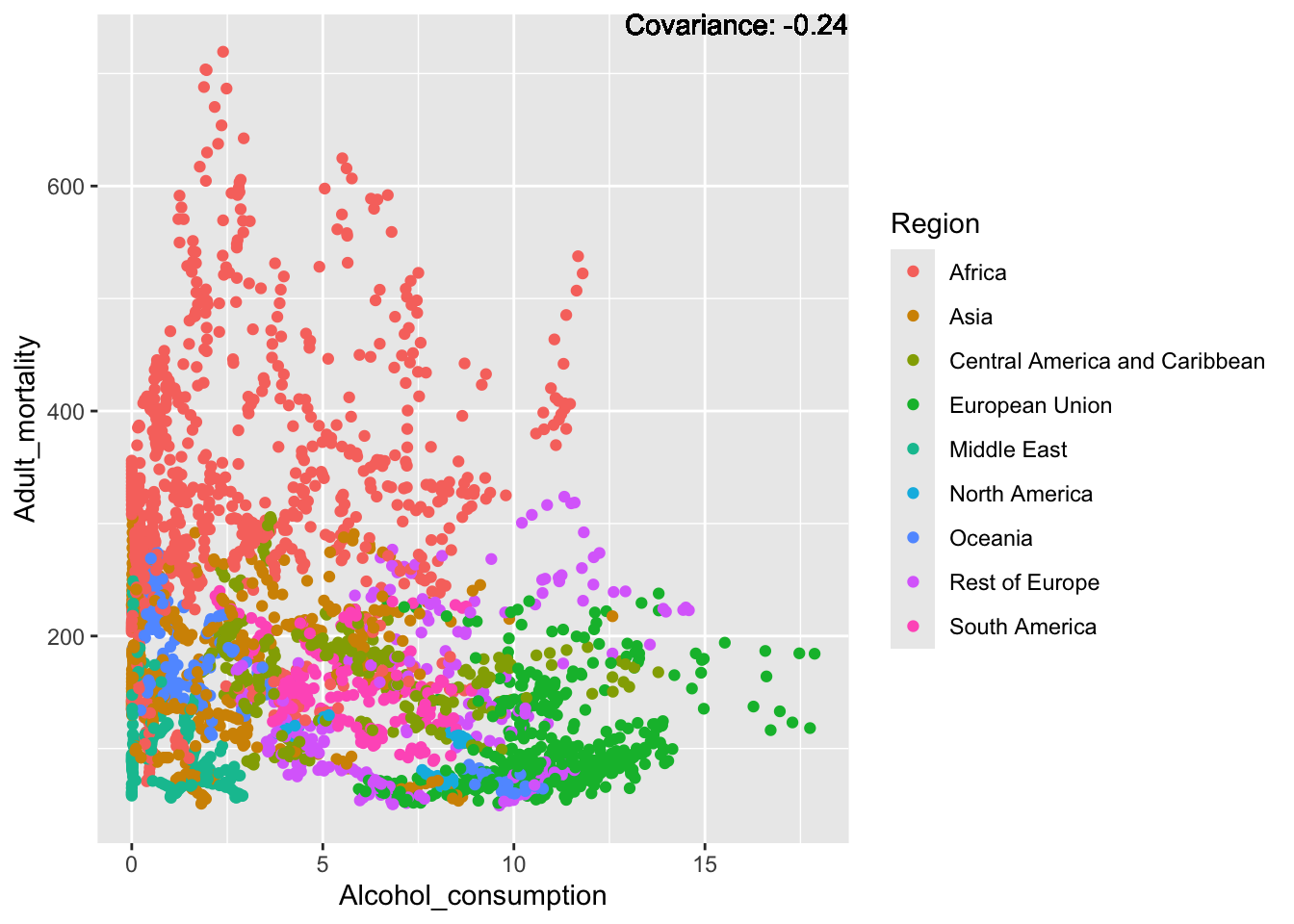

covariance_plot("Adult_mortality", "Population_mln", df, sdf)

Warning in geom_text(aes(label = paste("Covariance:", round(cov(std_data_frame[[y_val]], : All aesthetics have length 1, but the data has 2864 rows.
ℹ Please consider using `annotate()` or provide this layer with data containing
  a single row.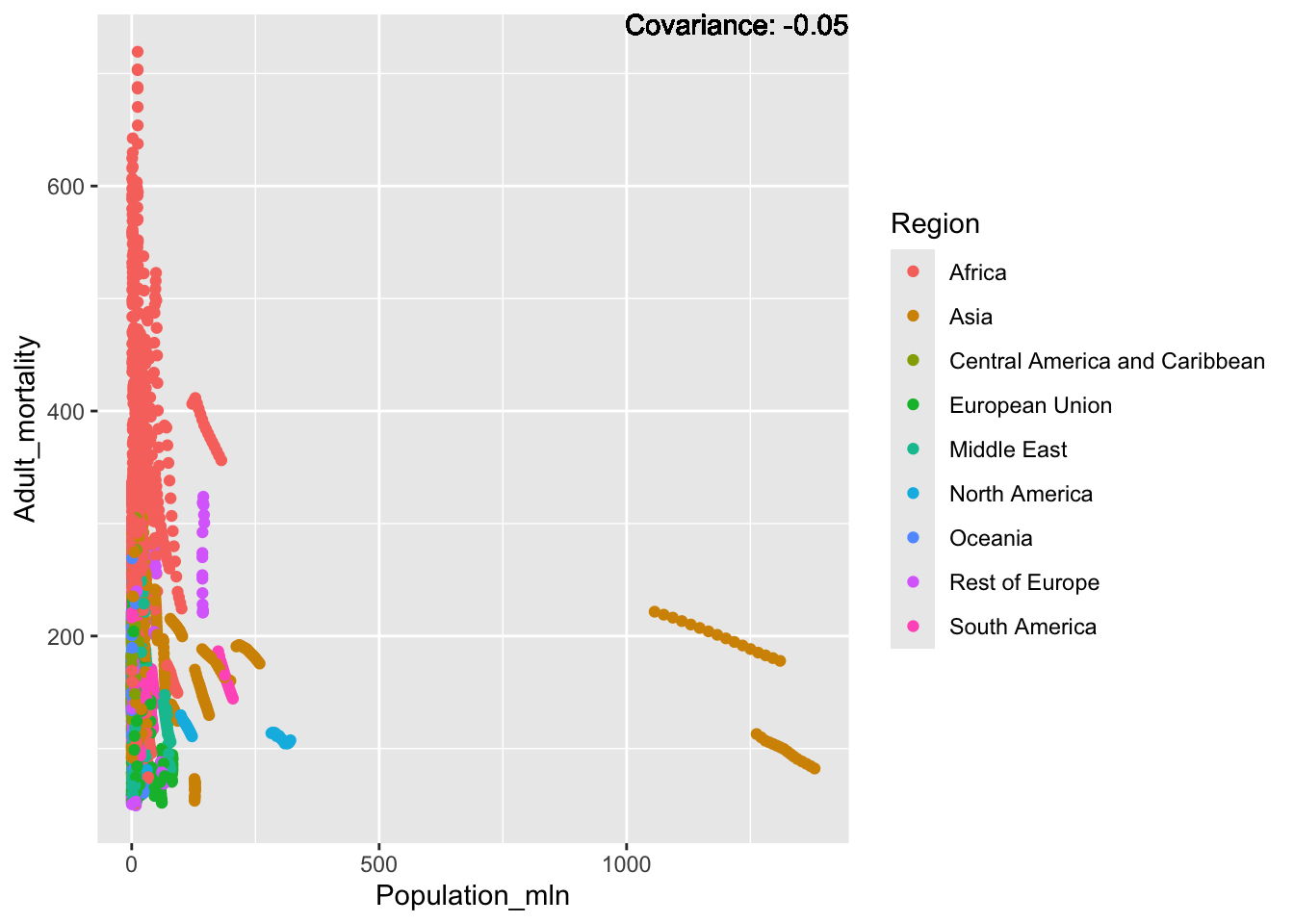

covariance_plot("Adult_mortality", "Thinness_ten_nineteen_years", df, sdf)

Warning in geom_text(aes(label = paste("Covariance:", round(cov(std_data_frame[[y_val]], : All aesthetics have length 1, but the data has 2864 rows.
ℹ Please consider using `annotate()` or provide this layer with data containing
  a single row.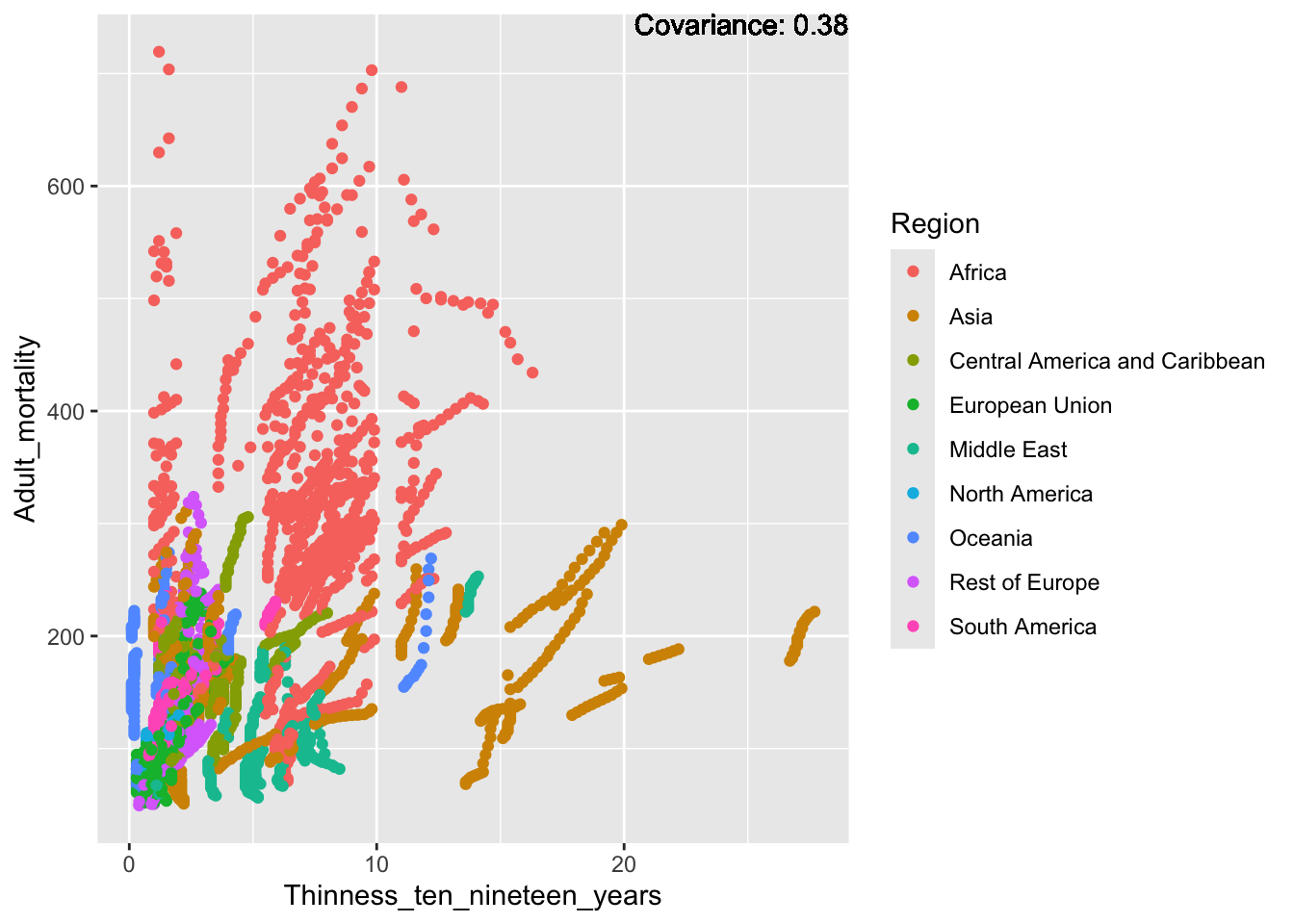

covariance_plot("Adult_mortality", "Thinness_five_nine_years", df, sdf)

Warning in geom_text(aes(label = paste("Covariance:", round(cov(std_data_frame[[y_val]], : All aesthetics have length 1, but the data has 2864 rows.
ℹ Please consider using `annotate()` or provide this layer with data containing
  a single row.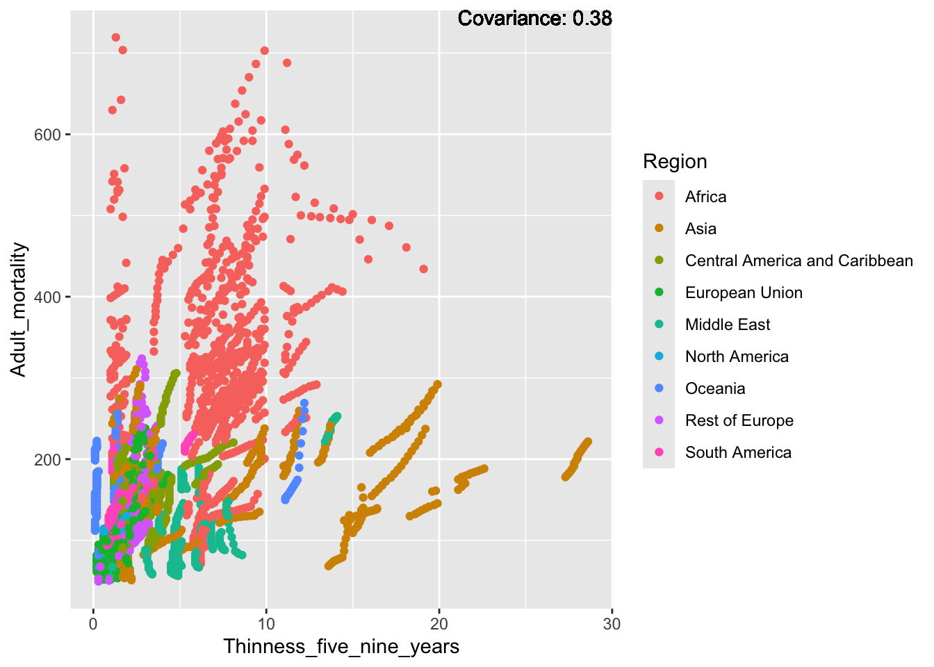

covariance_plot("Adult_mortality", "Schooling", df, sdf)

Warning in geom_text(aes(label = paste("Covariance:", round(cov(std_data_frame[[y_val]], : All aesthetics have length 1, but the data has 2864 rows.
ℹ Please consider using `annotate()` or provide this layer with data containing
  a single row.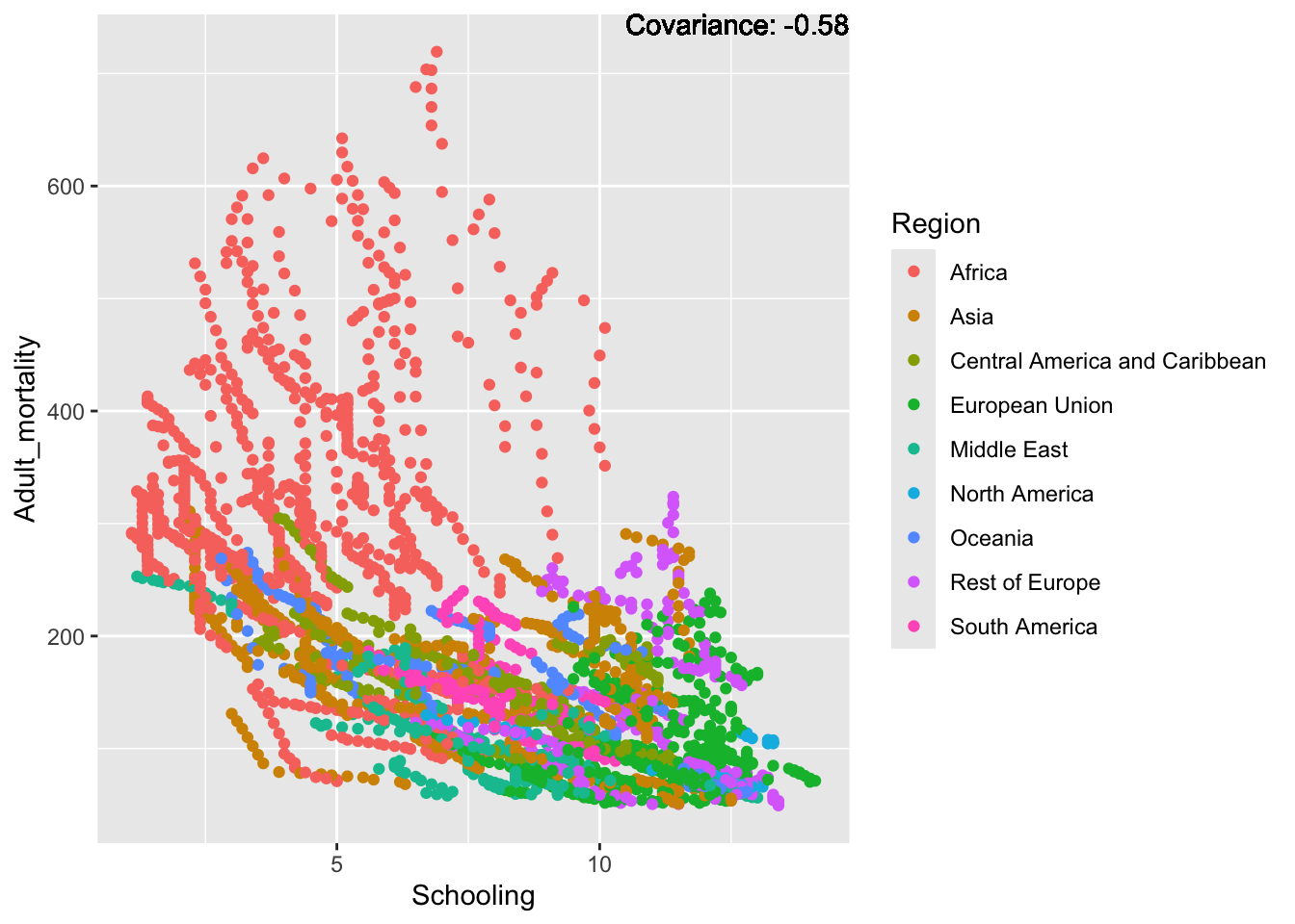

Inferences:

Strong negative: Life expectancy

Negative: BMI, polio Diphtheria, schooling

Positive: HIV

Strong positive: infant deaths, under five deaths

Hepatitis B:

covariance_plot("Hepatitis_B", "GDP_per_capita", df, sdf)

Warning in geom_text(aes(label = paste("Covariance:", round(cov(std_data_frame[[y_val]], : All aesthetics have length 1, but the data has 2864 rows.
ℹ Please consider using `annotate()` or provide this layer with data containing
  a single row.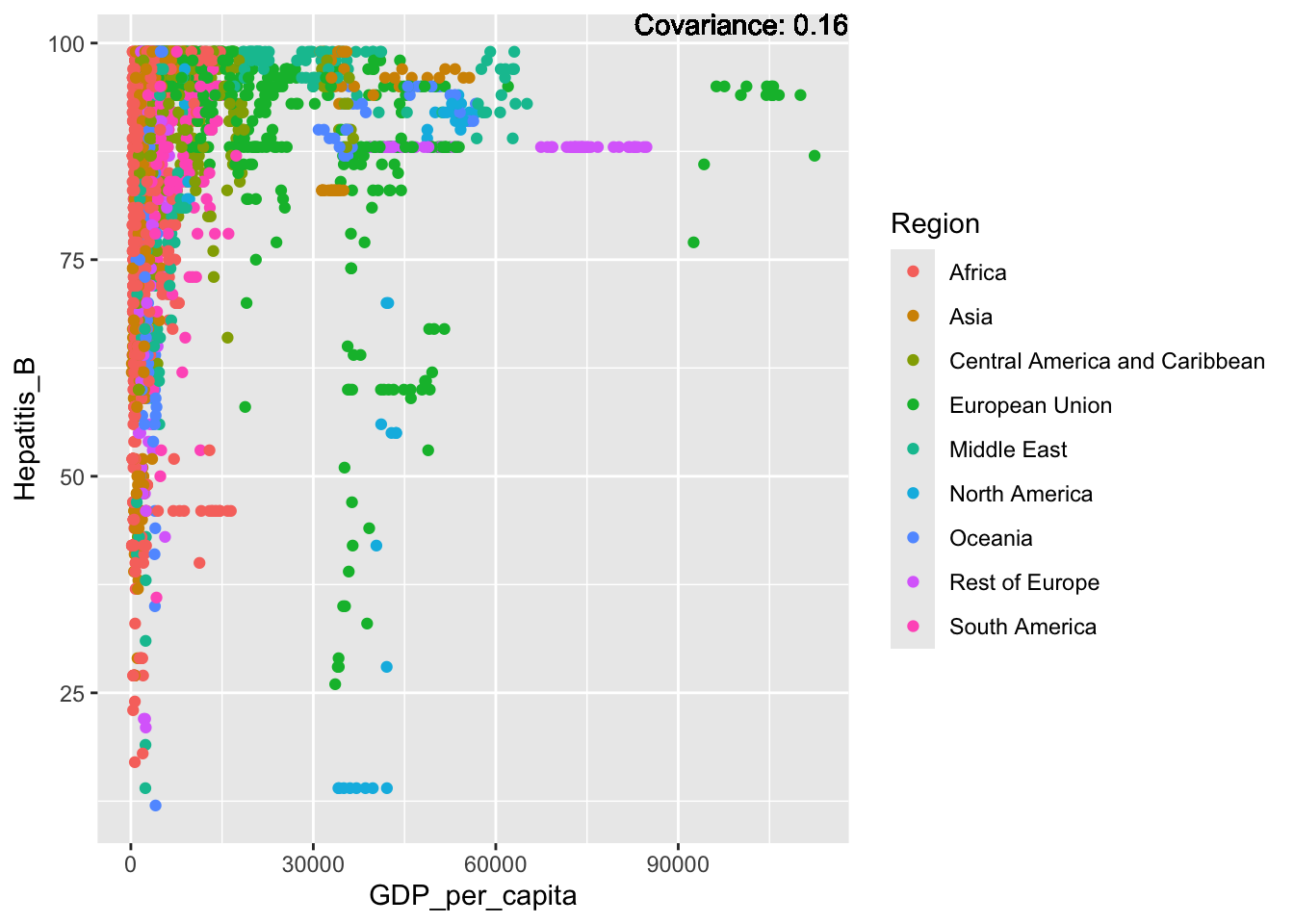

covariance_plot("Hepatitis_B", "Infant_deaths", df, sdf)

Warning in geom_text(aes(label = paste("Covariance:", round(cov(std_data_frame[[y_val]], : All aesthetics have length 1, but the data has 2864 rows.
ℹ Please consider using `annotate()` or provide this layer with data containing
  a single row.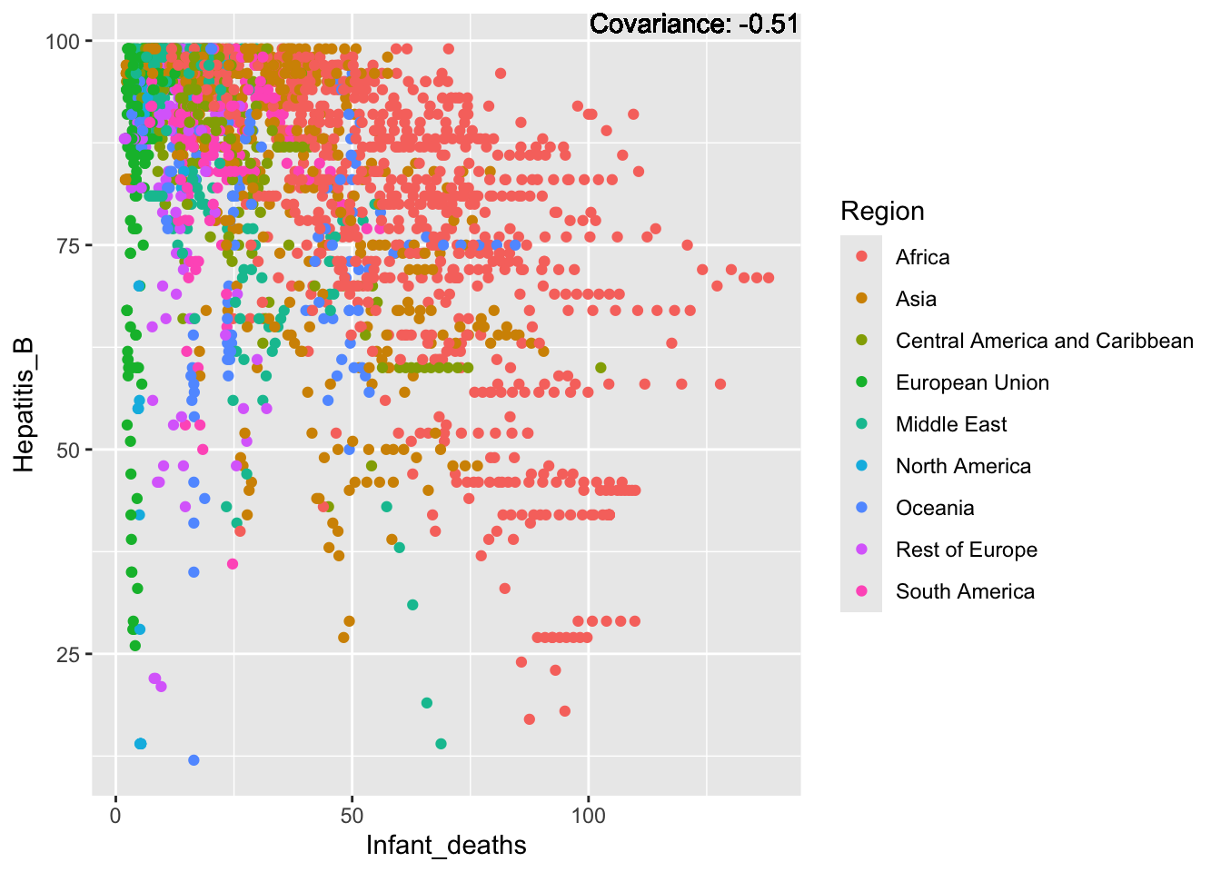

covariance_plot("Hepatitis_B", "Under_five_deaths", df, sdf)

Warning in geom_text(aes(label = paste("Covariance:", round(cov(std_data_frame[[y_val]], : All aesthetics have length 1, but the data has 2864 rows.
ℹ Please consider using `annotate()` or provide this layer with data containing
  a single row.

covariance_plot("Hepatitis_B", "Life_expectancy", df, sdf)

Warning in geom_text(aes(label = paste("Covariance:", round(cov(std_data_frame[[y_val]], : All aesthetics have length 1, but the data has 2864 rows.
ℹ Please consider using `annotate()` or provide this layer with data containing
  a single row.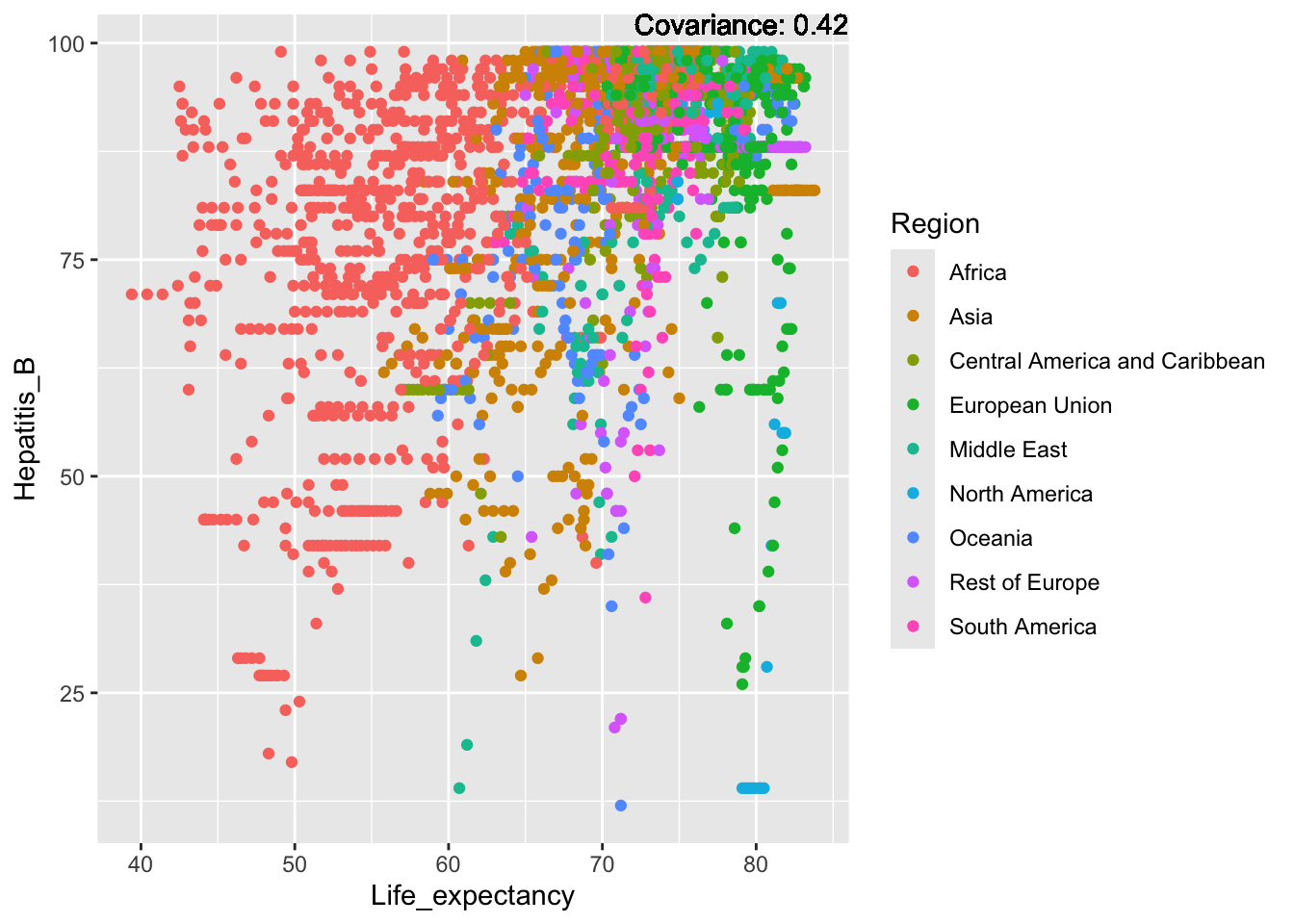

covariance_plot("Hepatitis_B", "Adult_mortality", df, sdf)

Warning in geom_text(aes(label = paste("Covariance:", round(cov(std_data_frame[[y_val]], : All aesthetics have length 1, but the data has 2864 rows.
ℹ Please consider using `annotate()` or provide this layer with data containing
  a single row.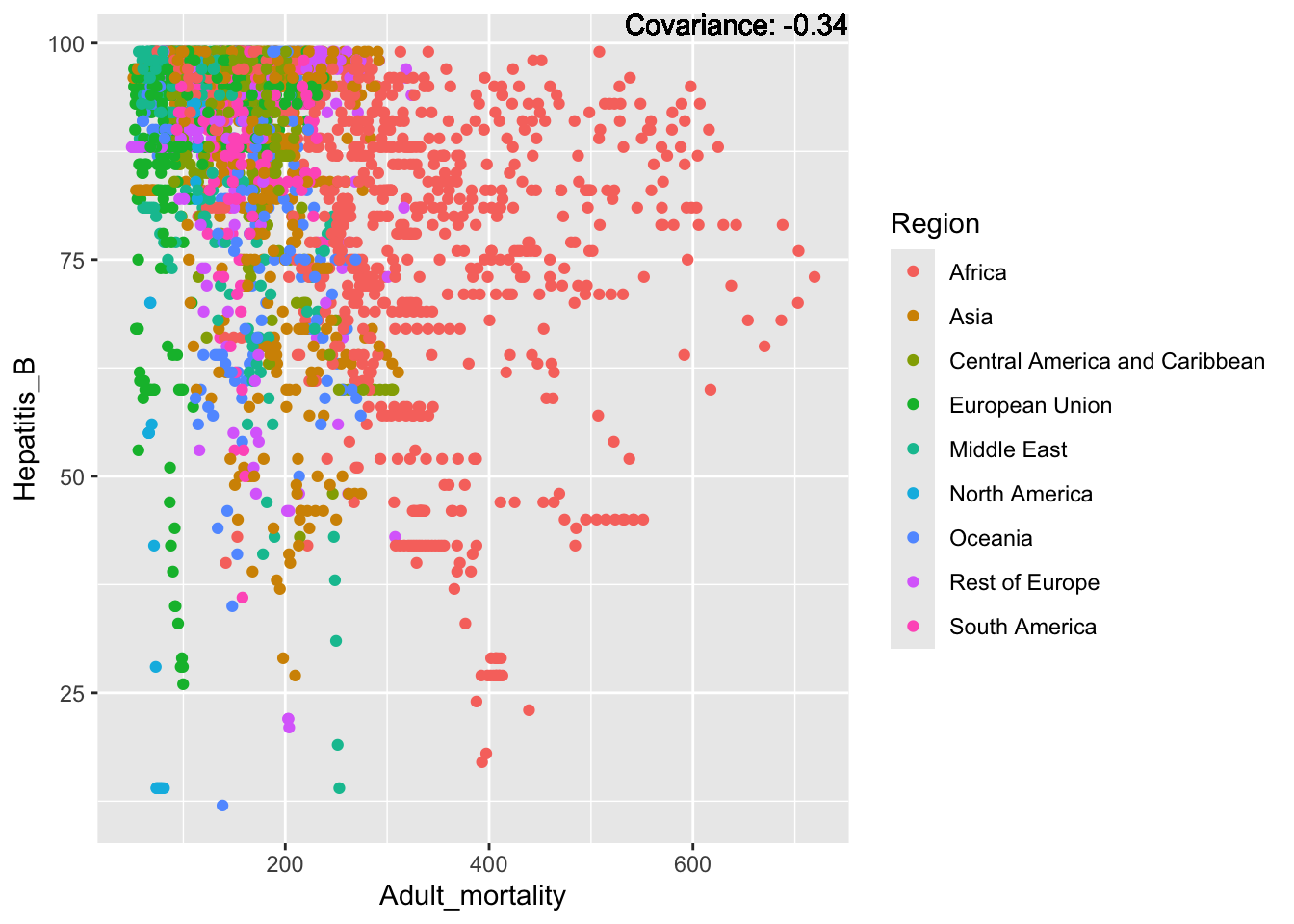

covariance_plot("Hepatitis_B", "Measles", df, sdf)

Warning in geom_text(aes(label = paste("Covariance:", round(cov(std_data_frame[[y_val]], : All aesthetics have length 1, but the data has 2864 rows.
ℹ Please consider using `annotate()` or provide this layer with data containing
  a single row.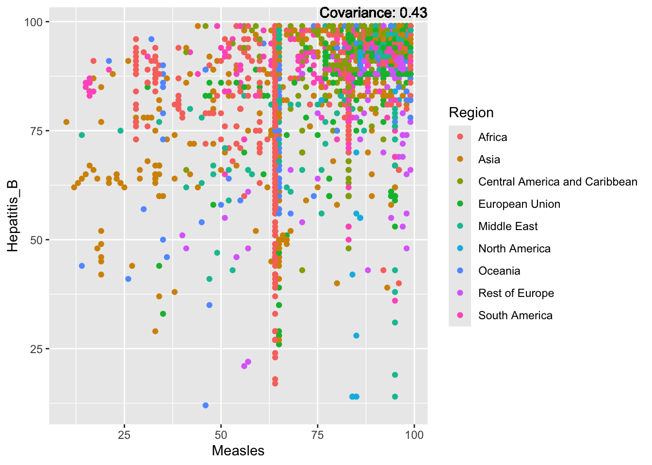

covariance_plot("Hepatitis_B", "BMI", df, sdf)

Warning in geom_text(aes(label = paste("Covariance:", round(cov(std_data_frame[[y_val]], : All aesthetics have length 1, but the data has 2864 rows.
ℹ Please consider using `annotate()` or provide this layer with data containing
  a single row.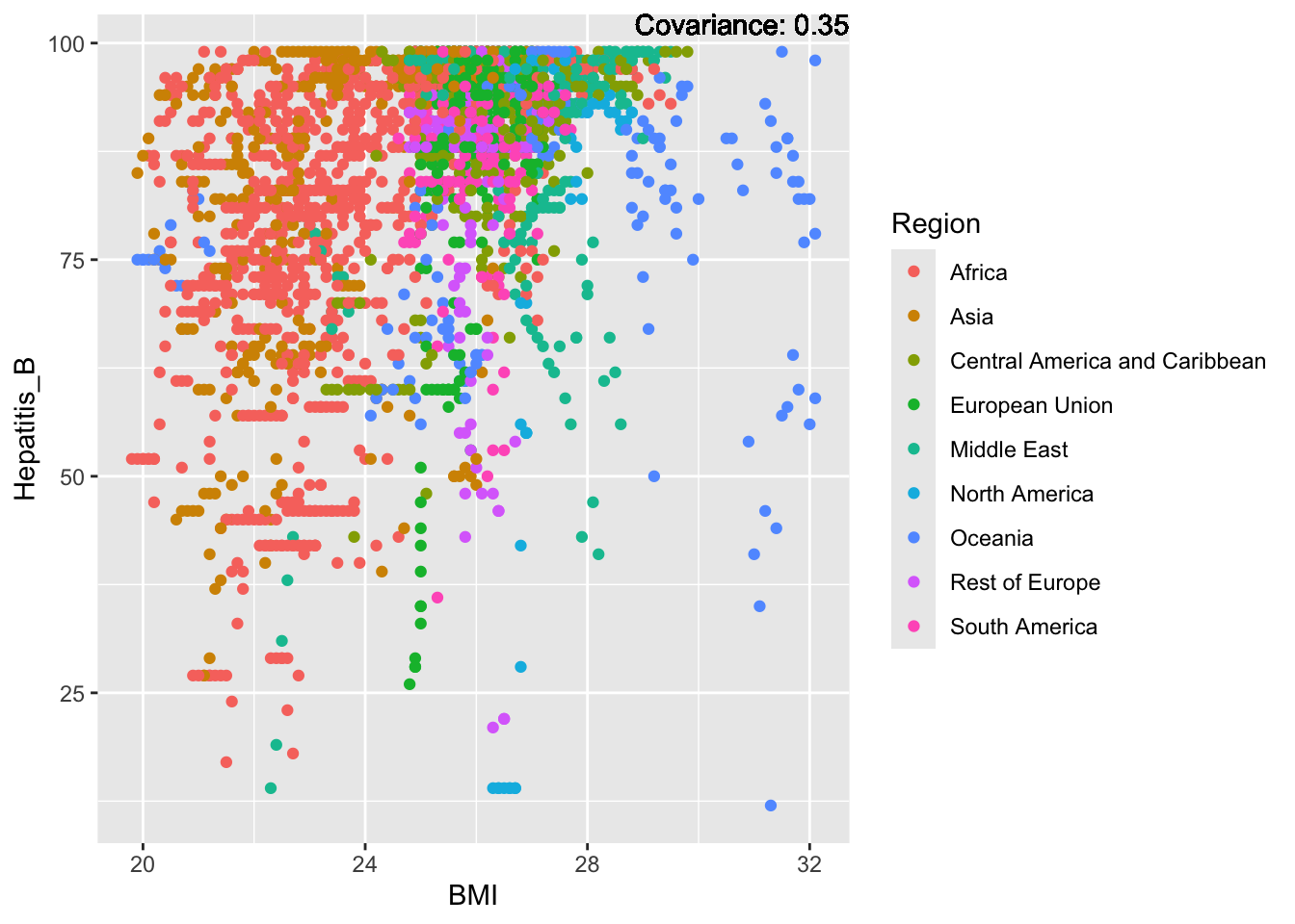

covariance_plot("Hepatitis_B", "Polio", df, sdf)

Warning in geom_text(aes(label = paste("Covariance:", round(cov(std_data_frame[[y_val]], : All aesthetics have length 1, but the data has 2864 rows.
ℹ Please consider using `annotate()` or provide this layer with data containing
  a single row.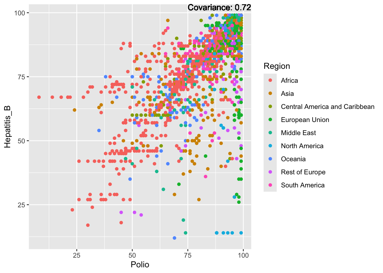

covariance_plot("Hepatitis_B", "Diphtheria", df, sdf)

Warning in geom_text(aes(label = paste("Covariance:", round(cov(std_data_frame[[y_val]], : All aesthetics have length 1, but the data has 2864 rows.
ℹ Please consider using `annotate()` or provide this layer with data containing
  a single row.

covariance_plot("Hepatitis_B", "Incidents_HIV", df, sdf)

Warning in geom_text(aes(label = paste("Covariance:", round(cov(std_data_frame[[y_val]], : All aesthetics have length 1, but the data has 2864 rows.
ℹ Please consider using `annotate()` or provide this layer with data containing
  a single row.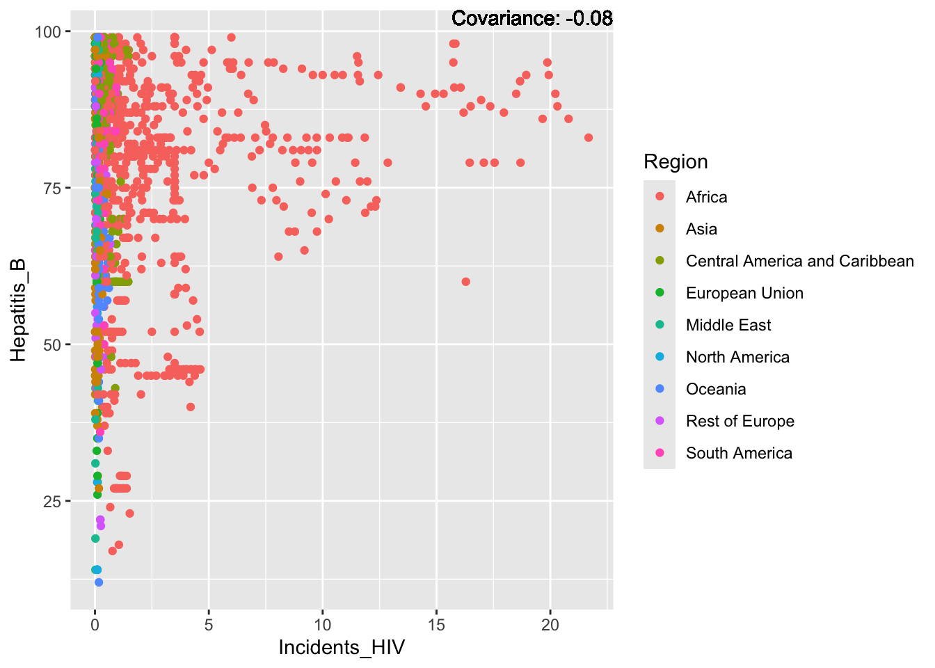

covariance_plot("Hepatitis_B", "Alcohol_consumption", df, sdf)

Warning in geom_text(aes(label = paste("Covariance:", round(cov(std_data_frame[[y_val]], : All aesthetics have length 1, but the data has 2864 rows.
ℹ Please consider using `annotate()` or provide this layer with data containing
  a single row.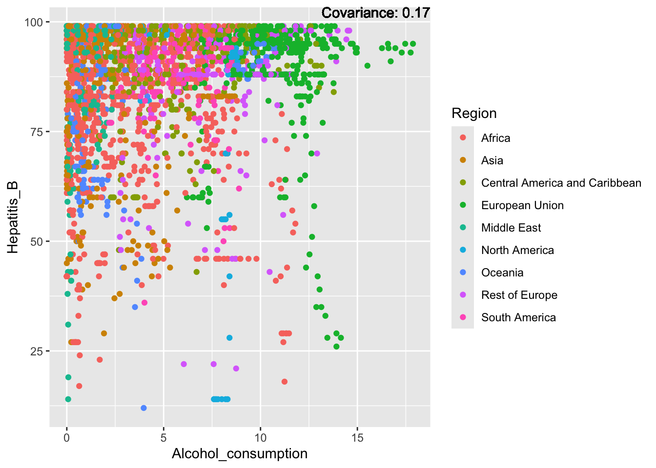

covariance_plot("Hepatitis_B", "Population_mln", df, sdf)

Warning in geom_text(aes(label = paste("Covariance:", round(cov(std_data_frame[[y_val]], : All aesthetics have length 1, but the data has 2864 rows.
ℹ Please consider using `annotate()` or provide this layer with data containing
  a single row.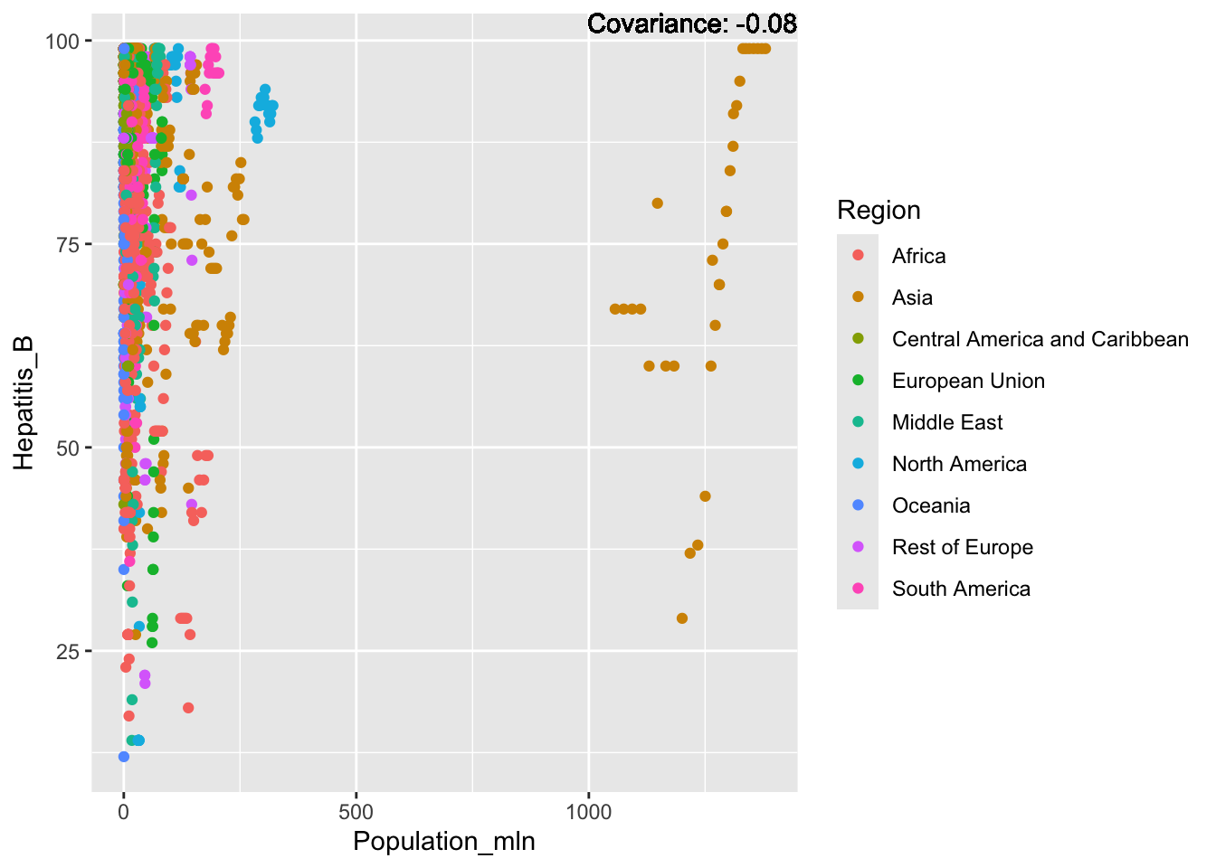

covariance_plot("Hepatitis_B", "Thinness_ten_nineteen_years", df, sdf)

Warning in geom_text(aes(label = paste("Covariance:", round(cov(std_data_frame[[y_val]], : All aesthetics have length 1, but the data has 2864 rows.
ℹ Please consider using `annotate()` or provide this layer with data containing
  a single row.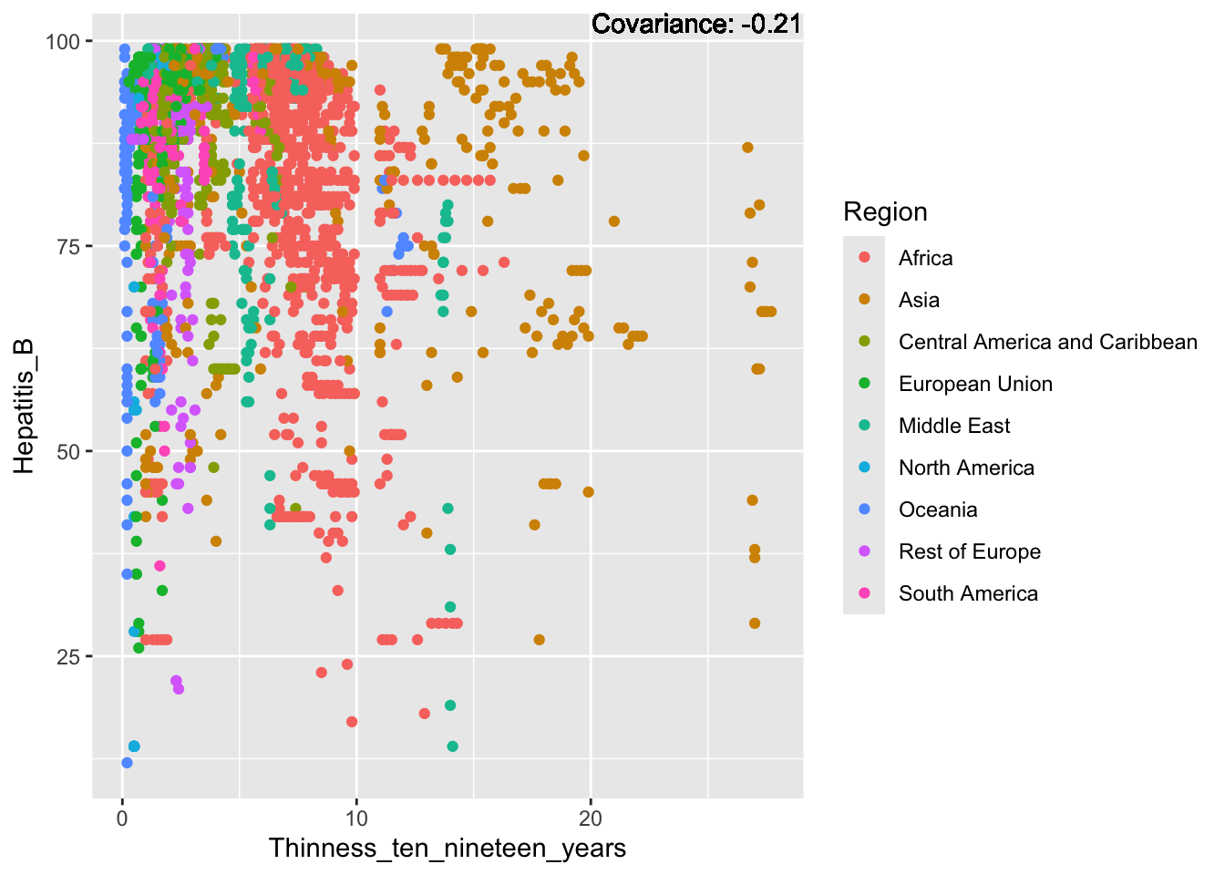

covariance_plot("Hepatitis_B", "Thinness_five_nine_years", df, sdf)

Warning in geom_text(aes(label = paste("Covariance:", round(cov(std_data_frame[[y_val]], : All aesthetics have length 1, but the data has 2864 rows.
ℹ Please consider using `annotate()` or provide this layer with data containing
  a single row.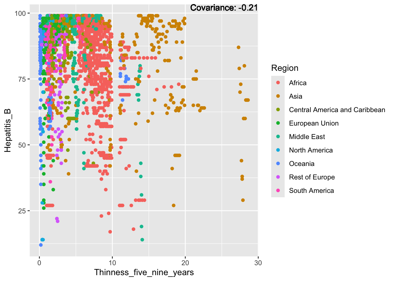

covariance_plot("Hepatitis_B", "Schooling", df, sdf)

Warning in geom_text(aes(label = paste("Covariance:", round(cov(std_data_frame[[y_val]], : All aesthetics have length 1, but the data has 2864 rows.
ℹ Please consider using `annotate()` or provide this layer with data containing
  a single row.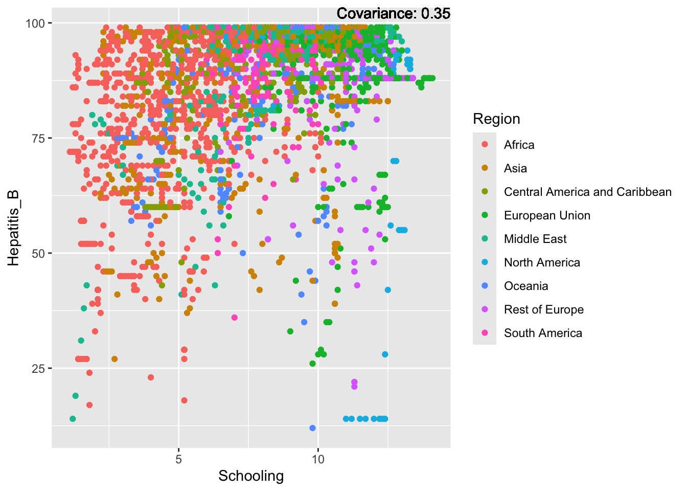

Hepatitis B Inferences:

Positive: Life Expectancy, Alcohol Consumption, Polio, Measles, Diphtheria

Negative: Infant Deaths, Under Five Deaths, Adult mortality

Measles:

covariance_plot("Measles", "GDP_per_capita", df, sdf)

Warning in geom_text(aes(label = paste("Covariance:", round(cov(std_data_frame[[y_val]], : All aesthetics have length 1, but the data has 2864 rows.
ℹ Please consider using `annotate()` or provide this layer with data containing
  a single row.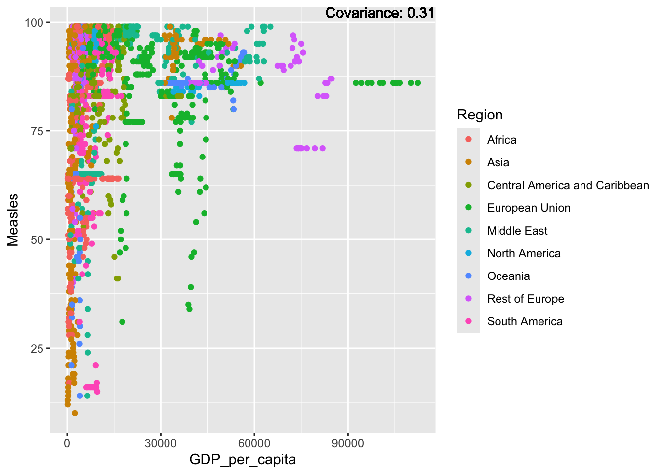

covariance_plot("Measles", "Infant_deaths", df, sdf)

Warning in geom_text(aes(label = paste("Covariance:", round(cov(std_data_frame[[y_val]], : All aesthetics have length 1, but the data has 2864 rows.
ℹ Please consider using `annotate()` or provide this layer with data containing
  a single row.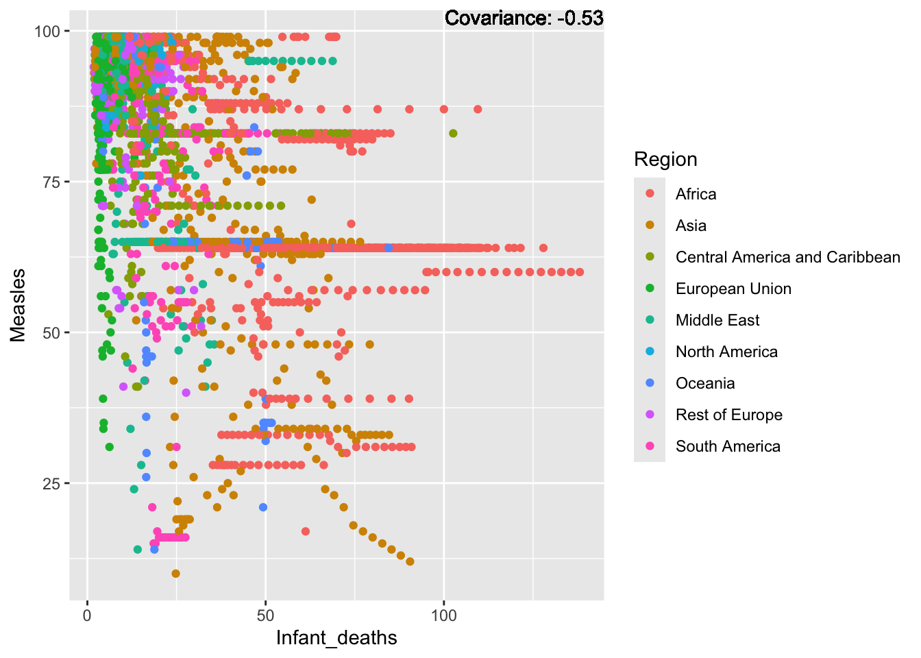

covariance_plot("Measles", "Under_five_deaths", df, sdf)

Warning in geom_text(aes(label = paste("Covariance:", round(cov(std_data_frame[[y_val]], : All aesthetics have length 1, but the data has 2864 rows.
ℹ Please consider using `annotate()` or provide this layer with data containing
  a single row.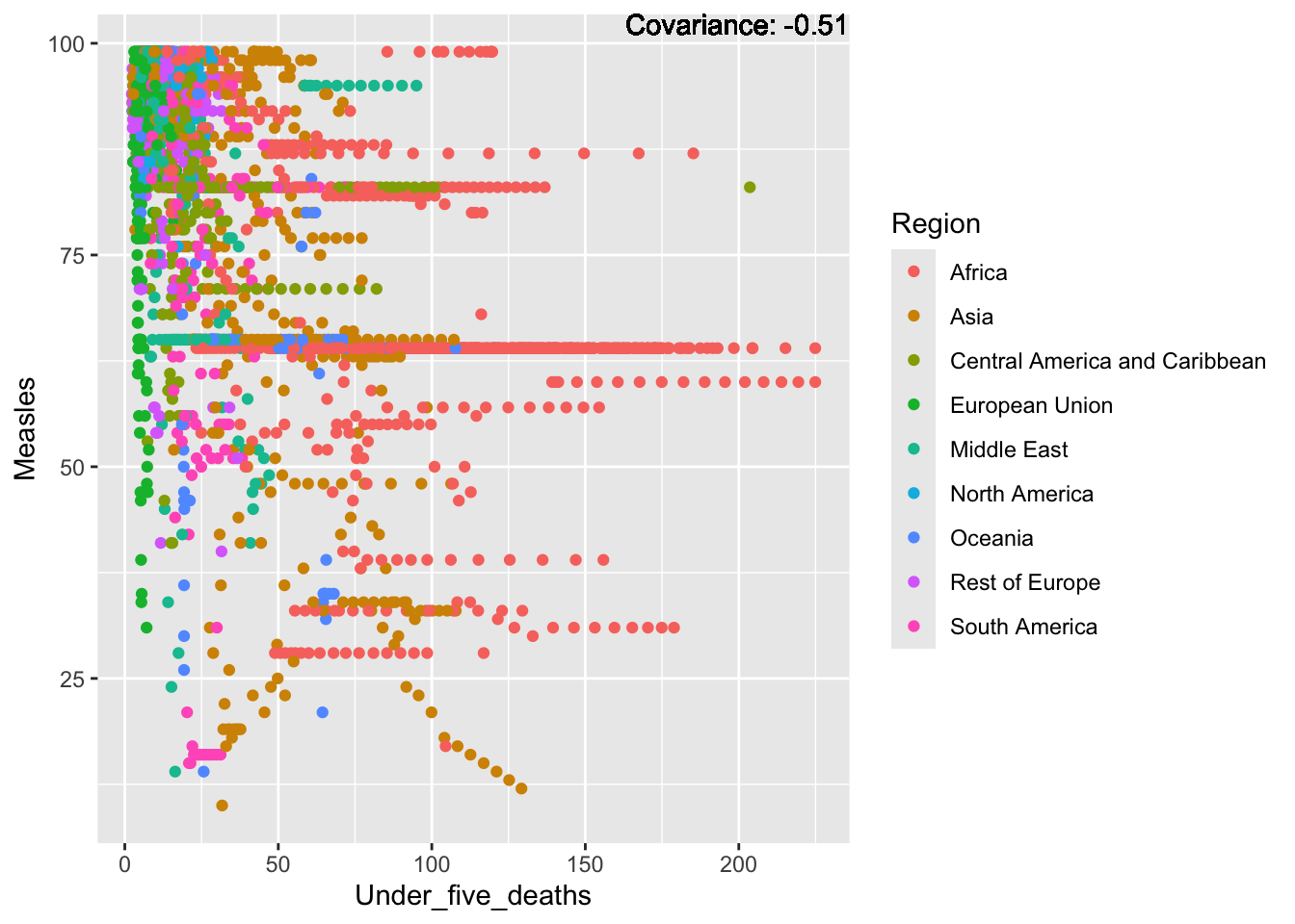

covariance_plot("Measles", "Life_expectancy", df, sdf)

Warning in geom_text(aes(label = paste("Covariance:", round(cov(std_data_frame[[y_val]], : All aesthetics have length 1, but the data has 2864 rows.
ℹ Please consider using `annotate()` or provide this layer with data containing
  a single row.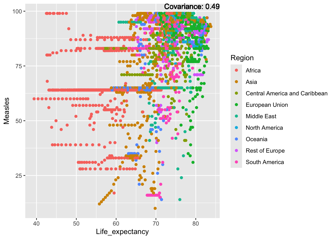

covariance_plot("Measles", "Adult_mortality", df, sdf)

Warning in geom_text(aes(label = paste("Covariance:", round(cov(std_data_frame[[y_val]], : All aesthetics have length 1, but the data has 2864 rows.
ℹ Please consider using `annotate()` or provide this layer with data containing
  a single row.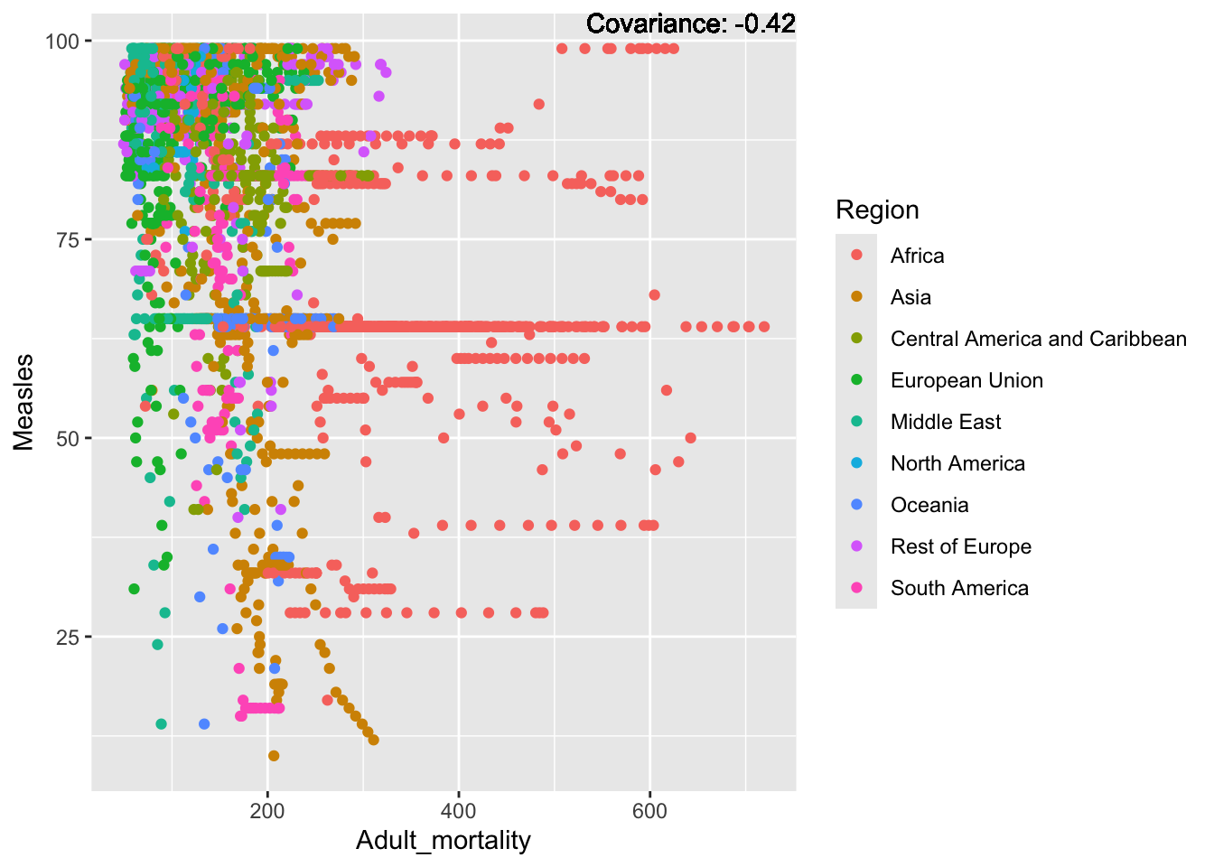

covariance_plot("Measles", "Hepatitis_B", df, sdf)

Warning in geom_text(aes(label = paste("Covariance:", round(cov(std_data_frame[[y_val]], : All aesthetics have length 1, but the data has 2864 rows.
ℹ Please consider using `annotate()` or provide this layer with data containing
  a single row.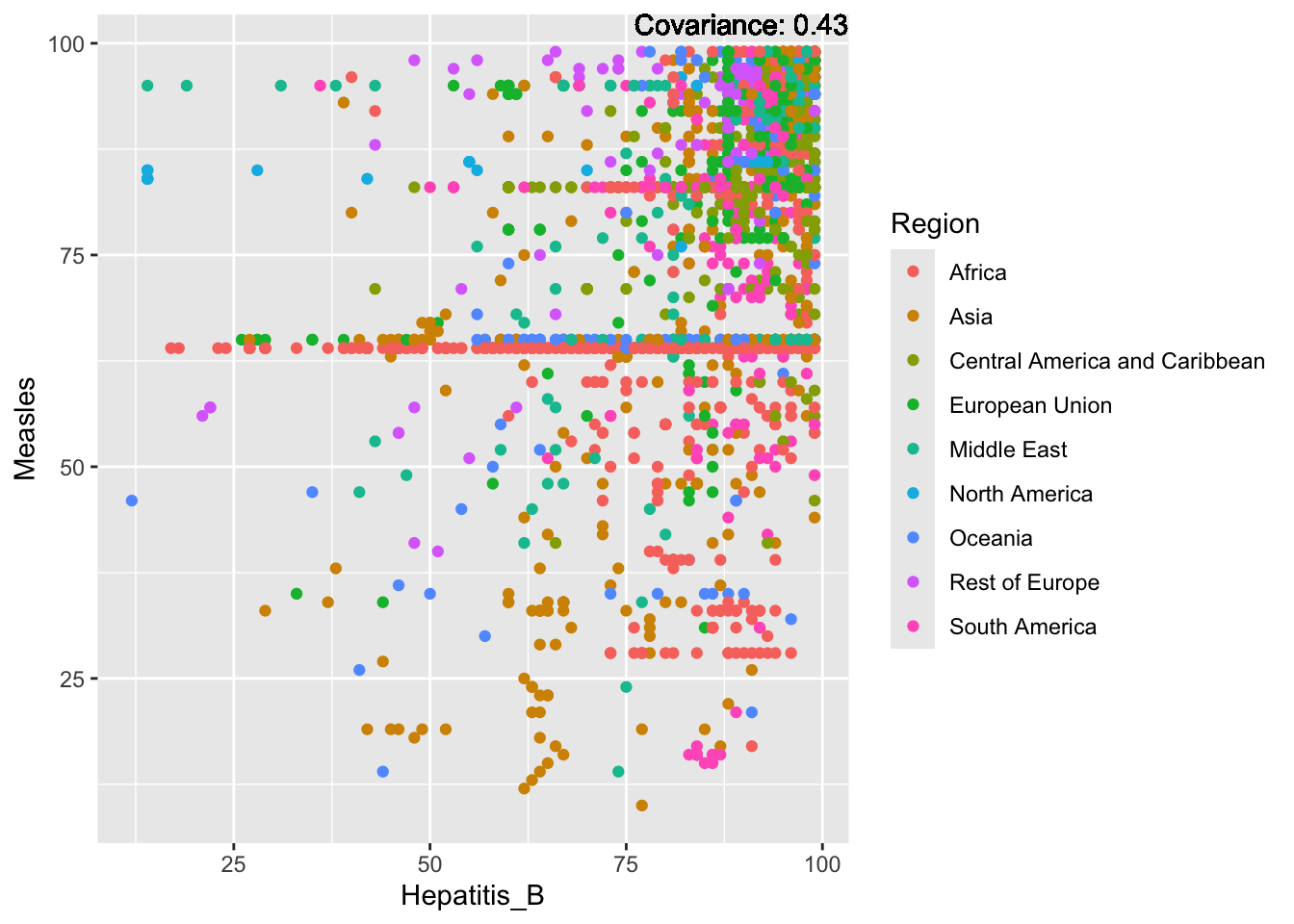

covariance_plot("Measles", "BMI", df, sdf)

Warning in geom_text(aes(label = paste("Covariance:", round(cov(std_data_frame[[y_val]], : All aesthetics have length 1, but the data has 2864 rows.
ℹ Please consider using `annotate()` or provide this layer with data containing
  a single row.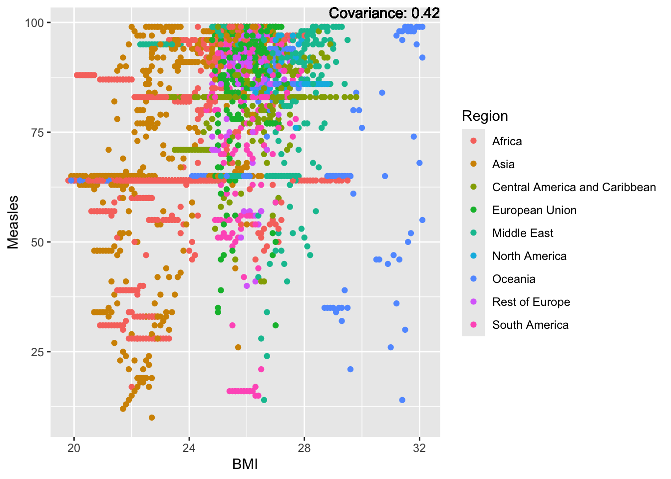

covariance_plot("Measles", "Polio", df, sdf)

Warning in geom_text(aes(label = paste("Covariance:", round(cov(std_data_frame[[y_val]], : All aesthetics have length 1, but the data has 2864 rows.
ℹ Please consider using `annotate()` or provide this layer with data containing
  a single row.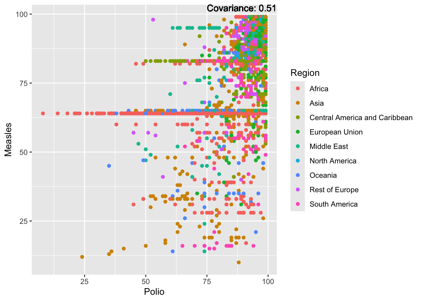

covariance_plot("Measles", "Diphtheria", df, sdf)

Warning in geom_text(aes(label = paste("Covariance:", round(cov(std_data_frame[[y_val]], : All aesthetics have length 1, but the data has 2864 rows.
ℹ Please consider using `annotate()` or provide this layer with data containing
  a single row.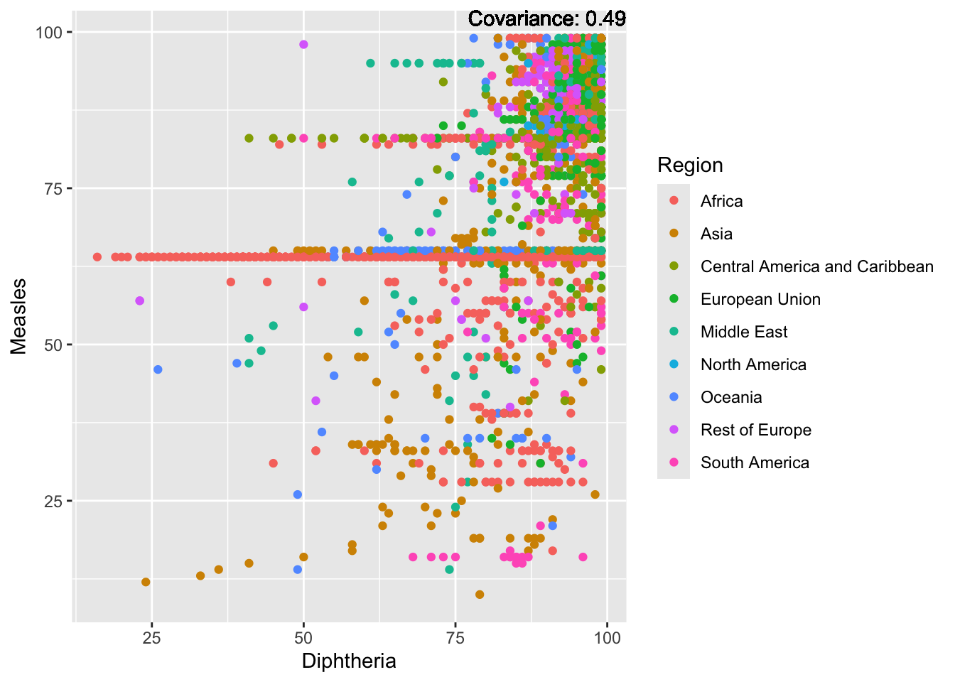

covariance_plot("Measles", "Incidents_HIV", df, sdf)

Warning in geom_text(aes(label = paste("Covariance:", round(cov(std_data_frame[[y_val]], : All aesthetics have length 1, but the data has 2864 rows.
ℹ Please consider using `annotate()` or provide this layer with data containing
  a single row.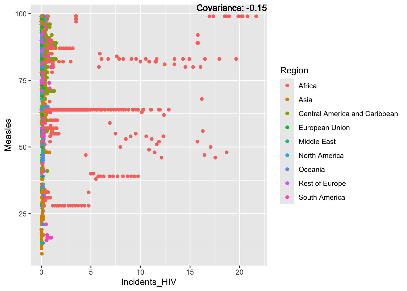

covariance_plot("Measles", "Alcohol_consumption", df, sdf)

Warning in geom_text(aes(label = paste("Covariance:", round(cov(std_data_frame[[y_val]], : All aesthetics have length 1, but the data has 2864 rows.
ℹ Please consider using `annotate()` or provide this layer with data containing
  a single row.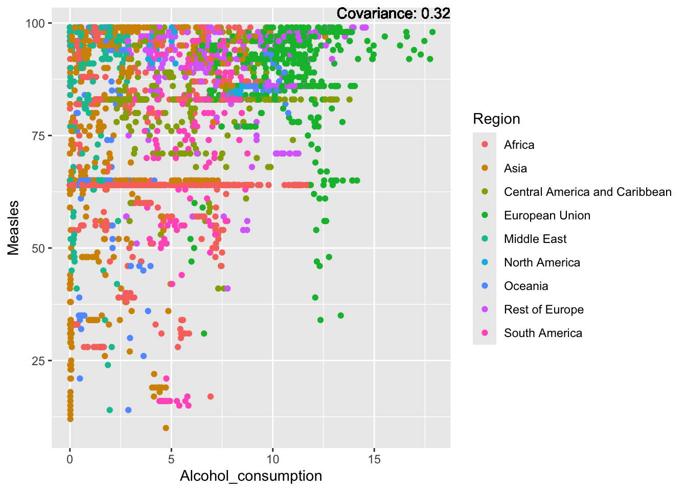

covariance_plot("Measles", "Population_mln", df, sdf)

Warning in geom_text(aes(label = paste("Covariance:", round(cov(std_data_frame[[y_val]], : All aesthetics have length 1, but the data has 2864 rows.
ℹ Please consider using `annotate()` or provide this layer with data containing
  a single row.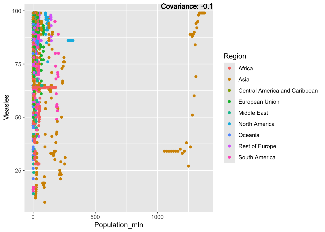

covariance_plot("Measles", "Thinness_ten_nineteen_years", df, sdf)

Warning in geom_text(aes(label = paste("Covariance:", round(cov(std_data_frame[[y_val]], : All aesthetics have length 1, but the data has 2864 rows.
ℹ Please consider using `annotate()` or provide this layer with data containing
  a single row.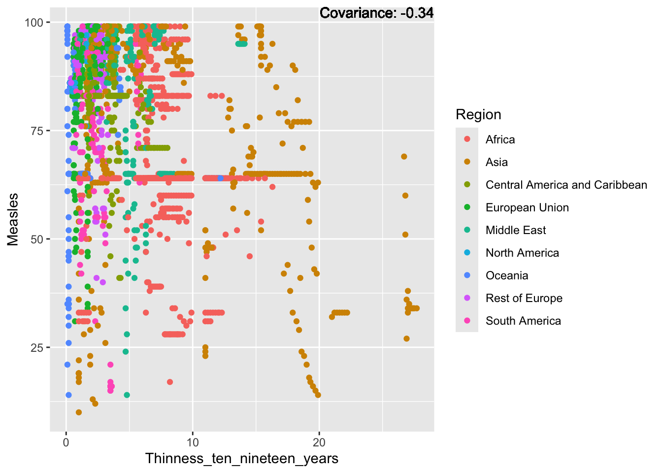

covariance_plot("Measles", "Thinness_five_nine_years", df, sdf)

Warning in geom_text(aes(label = paste("Covariance:", round(cov(std_data_frame[[y_val]], : All aesthetics have length 1, but the data has 2864 rows.
ℹ Please consider using `annotate()` or provide this layer with data containing
  a single row.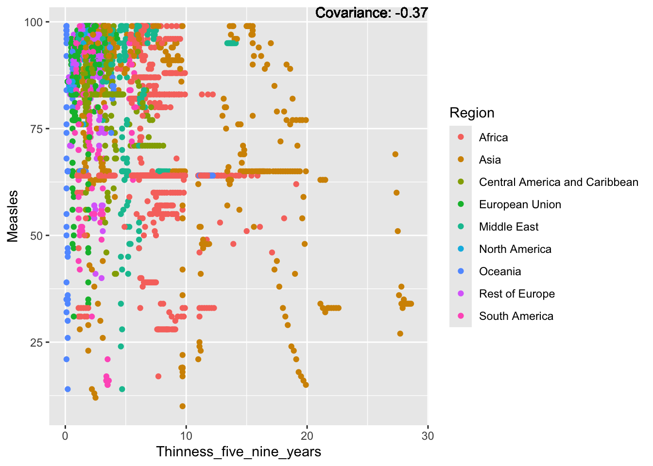

covariance_plot("Measles", "Schooling", df, sdf)

Warning in geom_text(aes(label = paste("Covariance:", round(cov(std_data_frame[[y_val]], : All aesthetics have length 1, but the data has 2864 rows.
ℹ Please consider using `annotate()` or provide this layer with data containing
  a single row.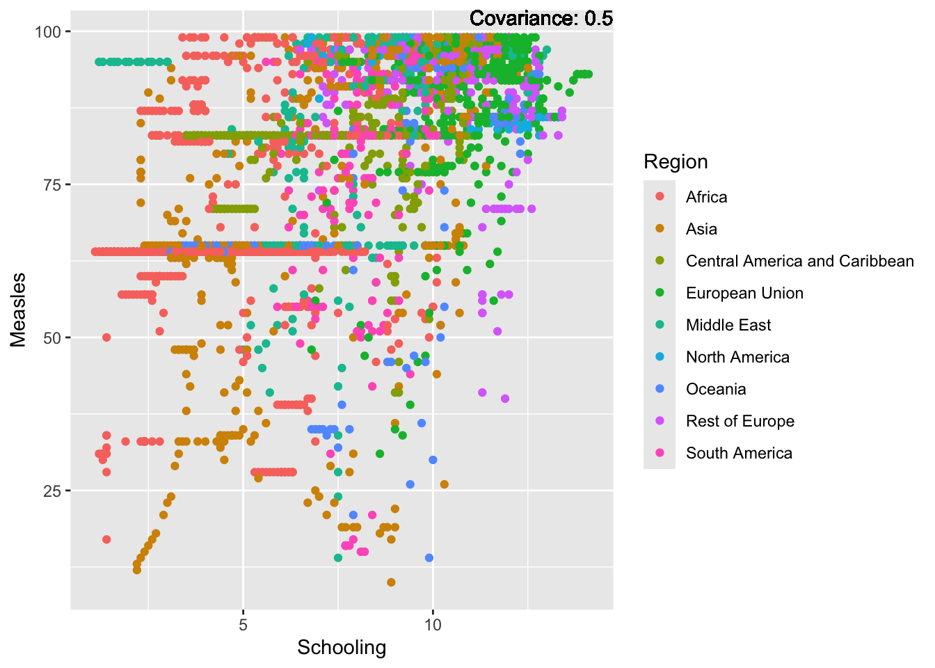

Measles Inferences:

Positive: Life Expectancy, Schooling, Hepatitis B, BMI, polio, Diphtheria

Negative: Infant Deaths, Under Five Deaths, adult mortality

BMI:

covariance_plot("BMI", "GDP_per_capita", df, sdf)

Warning in geom_text(aes(label = paste("Covariance:", round(cov(std_data_frame[[y_val]], : All aesthetics have length 1, but the data has 2864 rows.
ℹ Please consider using `annotate()` or provide this layer with data containing
  a single row.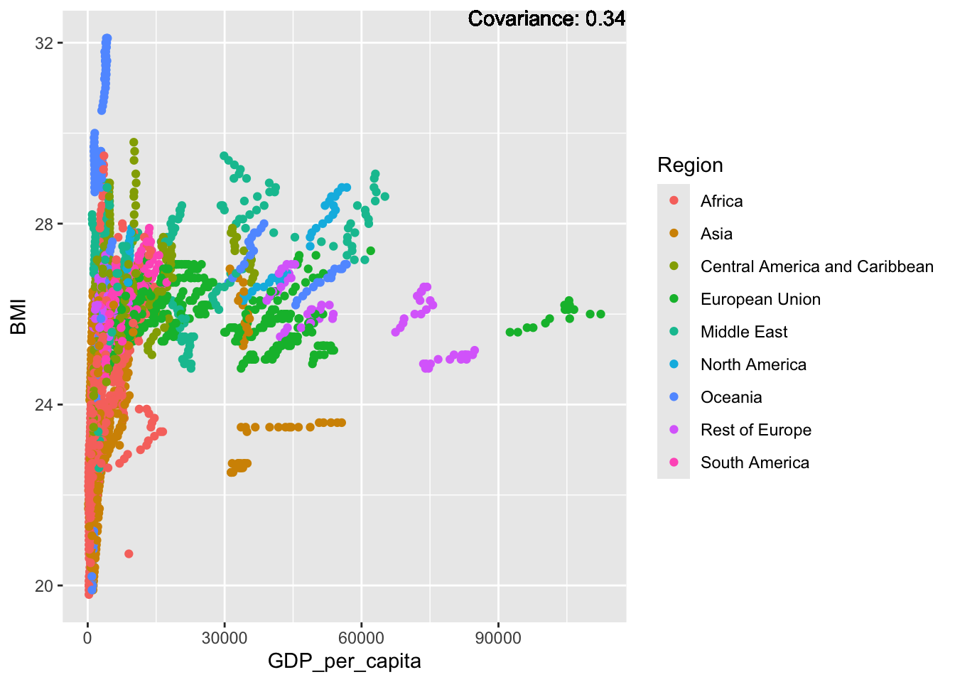

covariance_plot("BMI", "Infant_deaths", df, sdf)

Warning in geom_text(aes(label = paste("Covariance:", round(cov(std_data_frame[[y_val]], : All aesthetics have length 1, but the data has 2864 rows.
ℹ Please consider using `annotate()` or provide this layer with data containing
  a single row.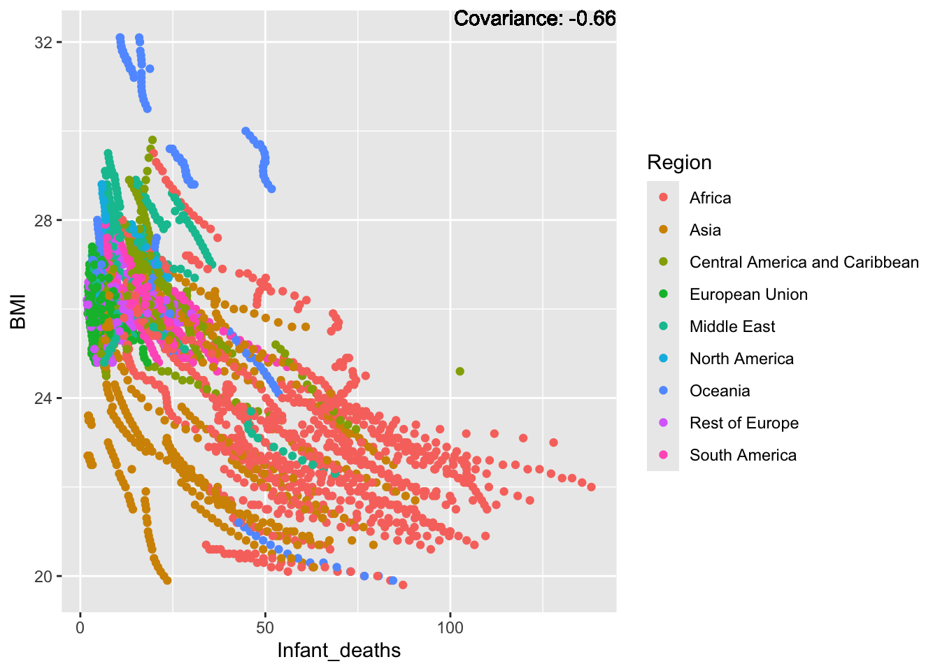

covariance_plot("BMI", "Under_five_deaths", df, sdf)

Warning in geom_text(aes(label = paste("Covariance:", round(cov(std_data_frame[[y_val]], : All aesthetics have length 1, but the data has 2864 rows.
ℹ Please consider using `annotate()` or provide this layer with data containing
  a single row.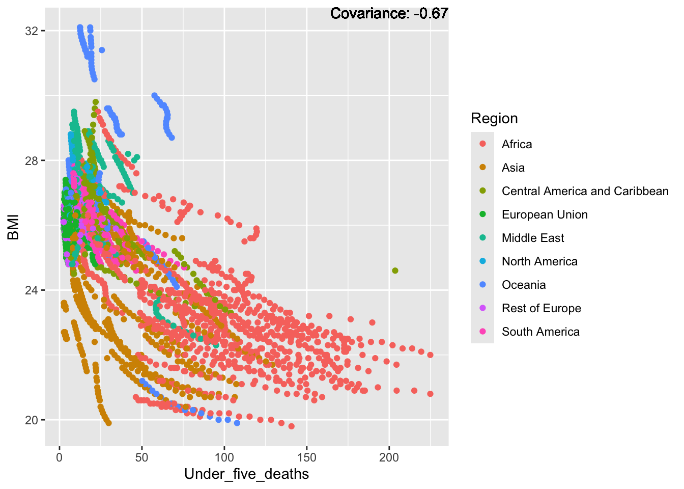

covariance_plot("BMI", "Life_expectancy", df, sdf)

Warning in geom_text(aes(label = paste("Covariance:", round(cov(std_data_frame[[y_val]], : All aesthetics have length 1, but the data has 2864 rows.
ℹ Please consider using `annotate()` or provide this layer with data containing
  a single row.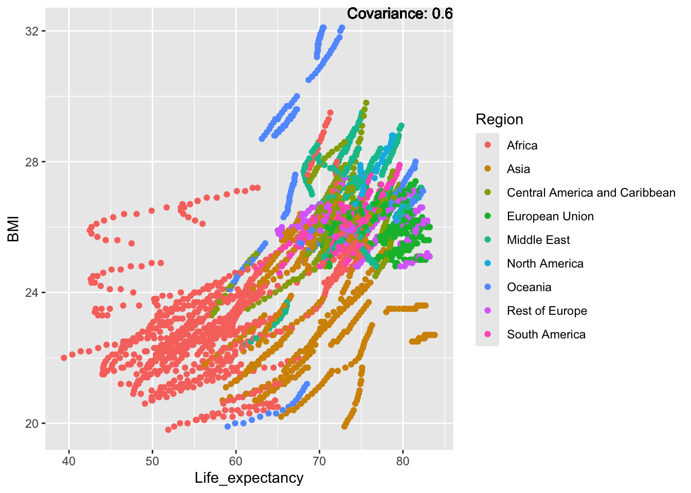

covariance_plot("BMI", "Adult_mortality", df, sdf)

Warning in geom_text(aes(label = paste("Covariance:", round(cov(std_data_frame[[y_val]], : All aesthetics have length 1, but the data has 2864 rows.
ℹ Please consider using `annotate()` or provide this layer with data containing
  a single row.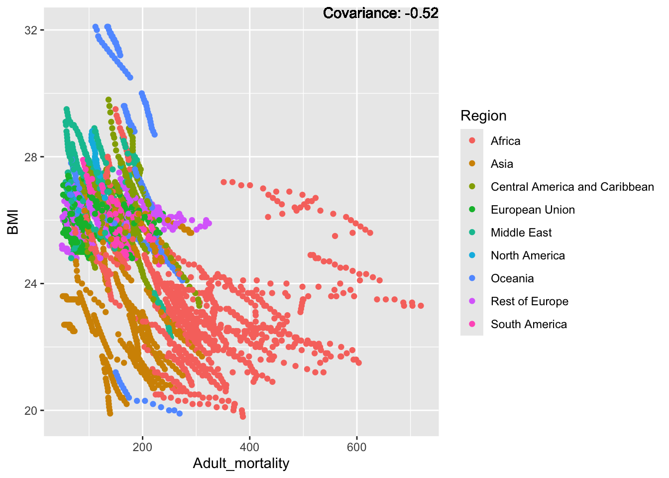

covariance_plot("BMI", "Hepatitis_B", df, sdf)

Warning in geom_text(aes(label = paste("Covariance:", round(cov(std_data_frame[[y_val]], : All aesthetics have length 1, but the data has 2864 rows.
ℹ Please consider using `annotate()` or provide this layer with data containing
  a single row.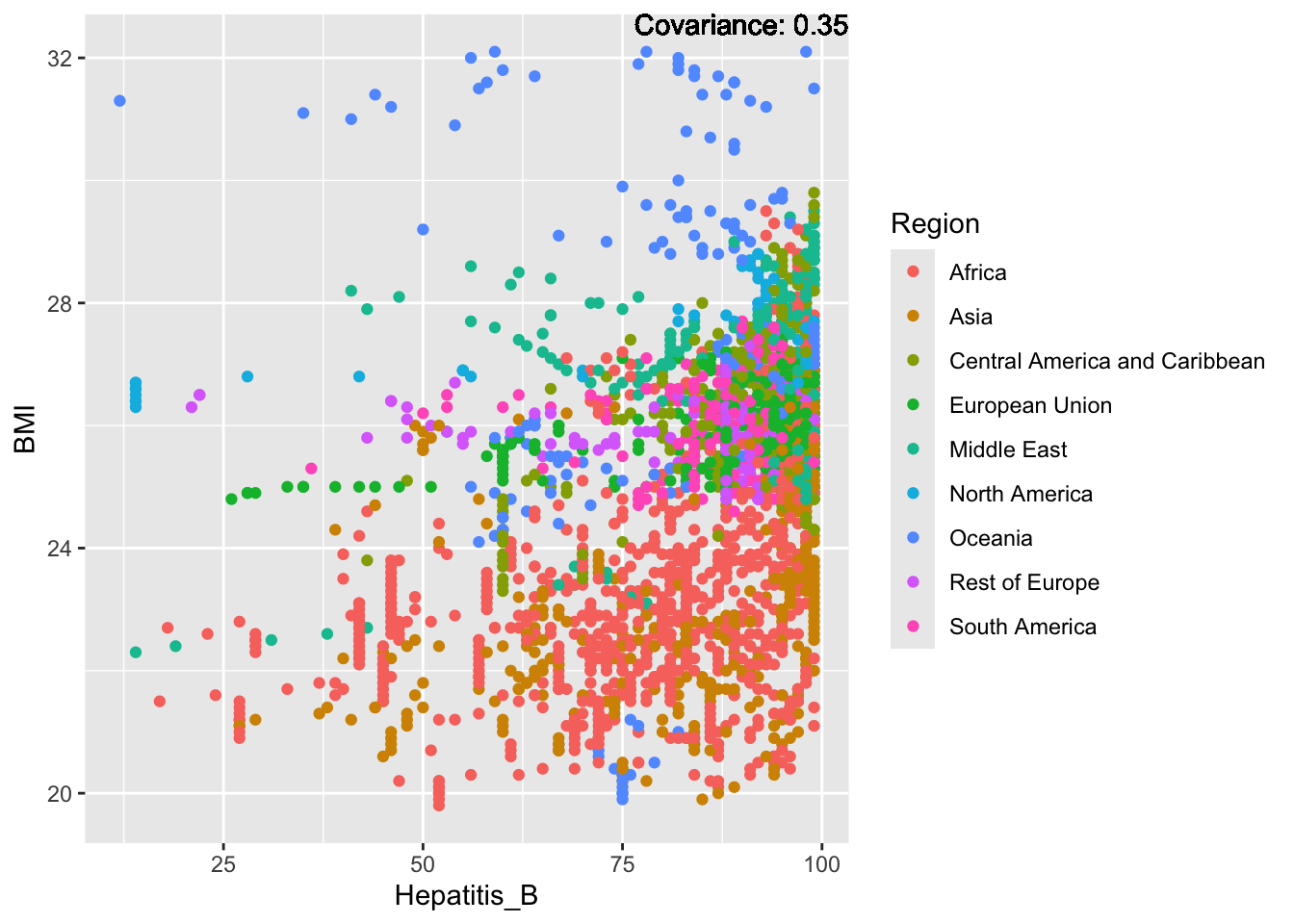

covariance_plot("BMI", "Measles", df, sdf)

Warning in geom_text(aes(label = paste("Covariance:", round(cov(std_data_frame[[y_val]], : All aesthetics have length 1, but the data has 2864 rows.
ℹ Please consider using `annotate()` or provide this layer with data containing
  a single row.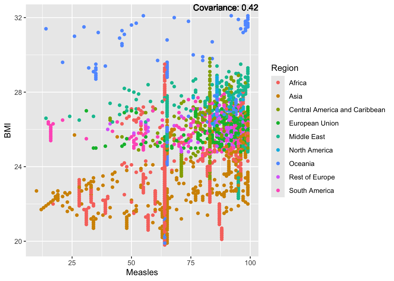

covariance_plot("BMI", "Polio", df, sdf)

Warning in geom_text(aes(label = paste("Covariance:", round(cov(std_data_frame[[y_val]], : All aesthetics have length 1, but the data has 2864 rows.
ℹ Please consider using `annotate()` or provide this layer with data containing
  a single row.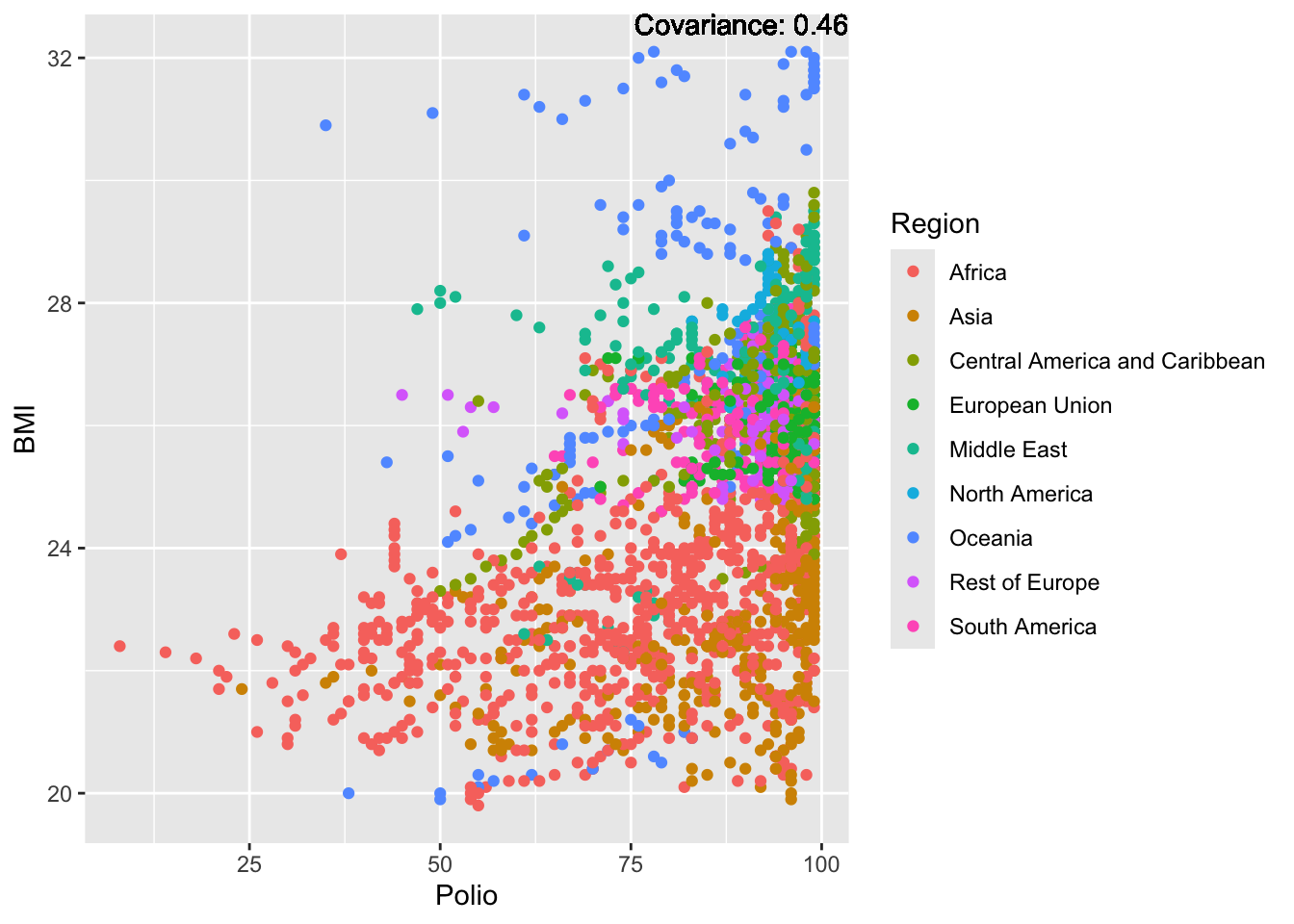

covariance_plot("BMI", "Diphtheria", df, sdf)

Warning in geom_text(aes(label = paste("Covariance:", round(cov(std_data_frame[[y_val]], : All aesthetics have length 1, but the data has 2864 rows.
ℹ Please consider using `annotate()` or provide this layer with data containing
  a single row.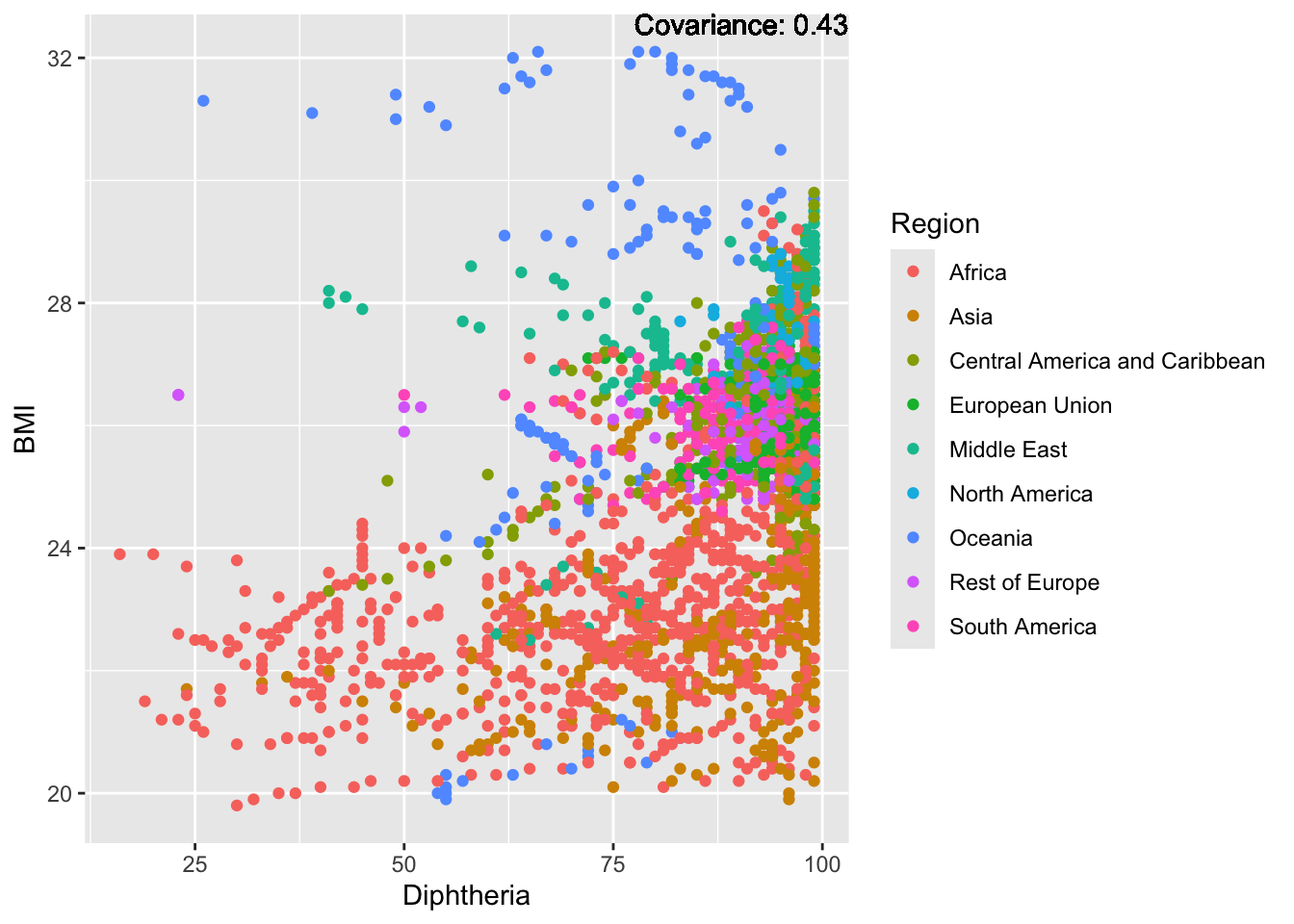

covariance_plot("BMI", "Incidents_HIV", df, sdf)

Warning in geom_text(aes(label = paste("Covariance:", round(cov(std_data_frame[[y_val]], : All aesthetics have length 1, but the data has 2864 rows.
ℹ Please consider using `annotate()` or provide this layer with data containing
  a single row.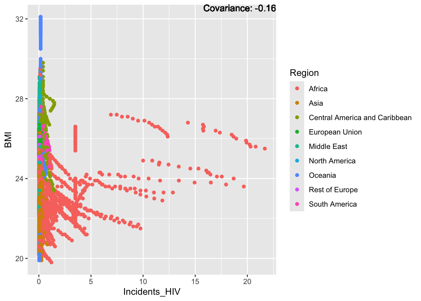

covariance_plot("BMI", "Alcohol_consumption", df, sdf)

Warning in geom_text(aes(label = paste("Covariance:", round(cov(std_data_frame[[y_val]], : All aesthetics have length 1, but the data has 2864 rows.
ℹ Please consider using `annotate()` or provide this layer with data containing
  a single row.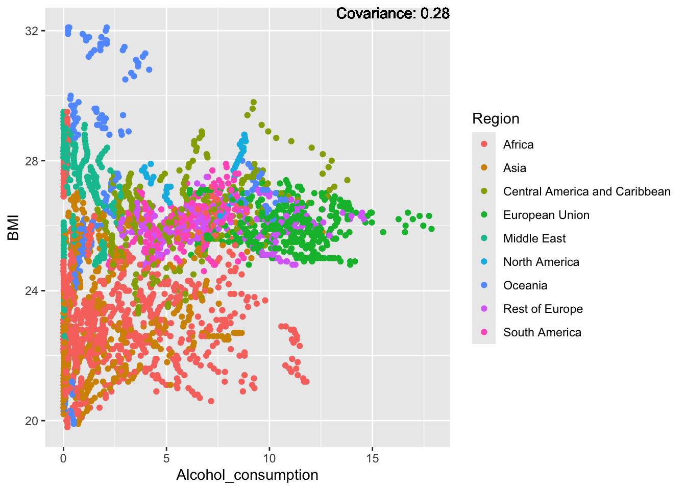

covariance_plot("BMI", "Population_mln", df, sdf)

Warning in geom_text(aes(label = paste("Covariance:", round(cov(std_data_frame[[y_val]], : All aesthetics have length 1, but the data has 2864 rows.
ℹ Please consider using `annotate()` or provide this layer with data containing
  a single row.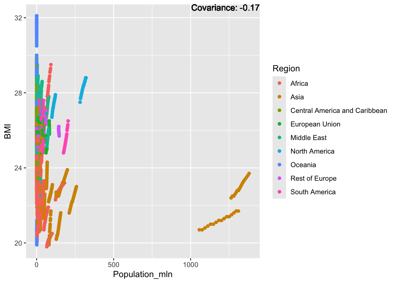

covariance_plot("BMI", "Thinness_ten_nineteen_years", df, sdf)

Warning in geom_text(aes(label = paste("Covariance:", round(cov(std_data_frame[[y_val]], : All aesthetics have length 1, but the data has 2864 rows.
ℹ Please consider using `annotate()` or provide this layer with data containing
  a single row.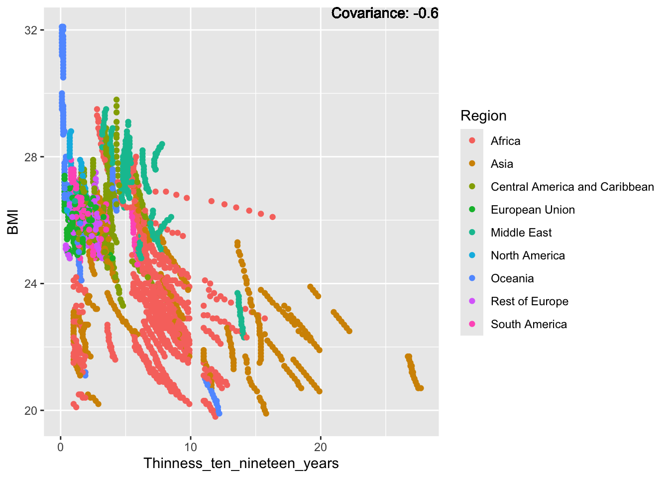

covariance_plot("BMI", "Thinness_five_nine_years", df, sdf)

Warning in geom_text(aes(label = paste("Covariance:", round(cov(std_data_frame[[y_val]], : All aesthetics have length 1, but the data has 2864 rows.
ℹ Please consider using `annotate()` or provide this layer with data containing
  a single row.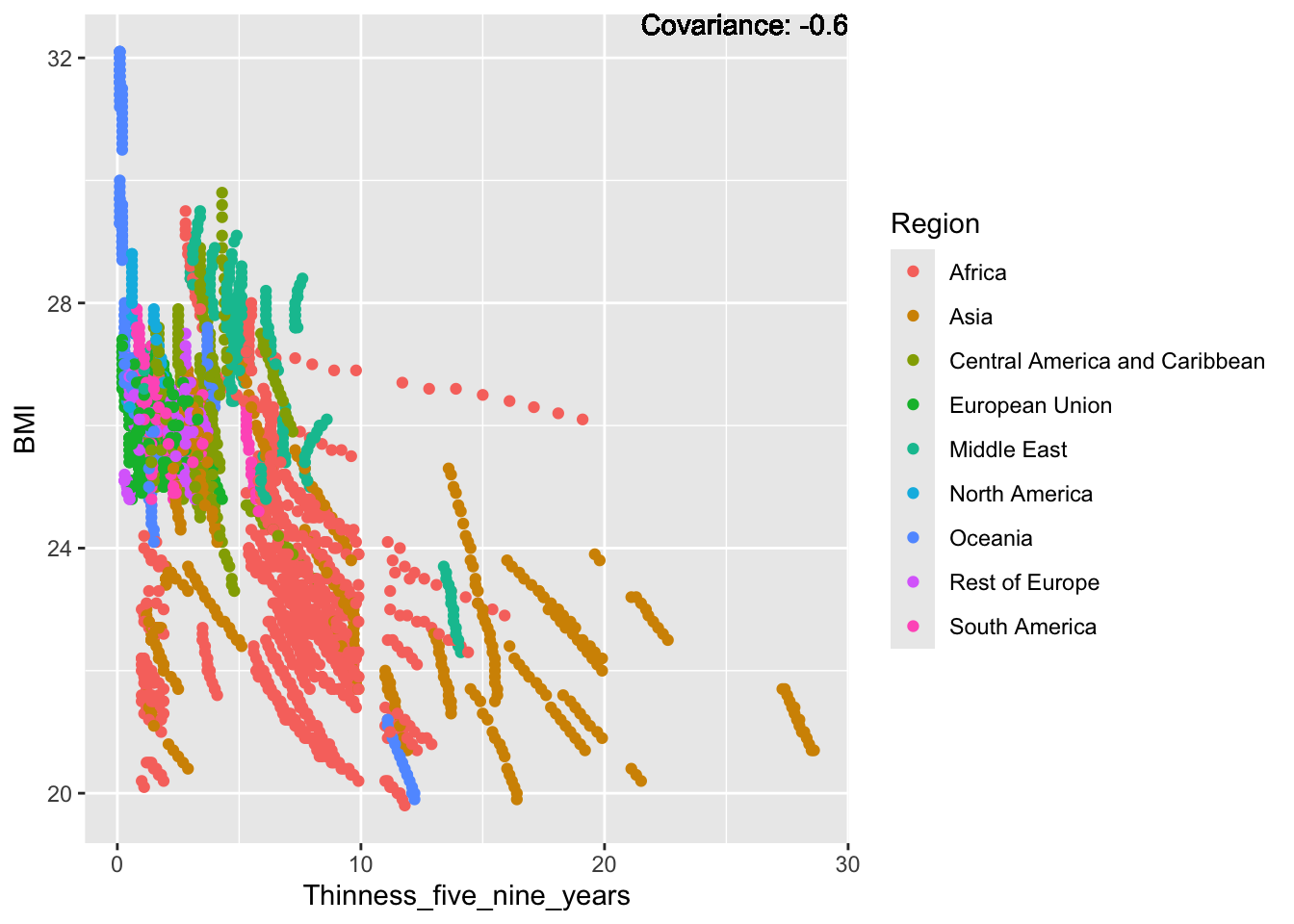

covariance_plot("BMI", "Schooling", df, sdf)

Warning in geom_text(aes(label = paste("Covariance:", round(cov(std_data_frame[[y_val]], : All aesthetics have length 1, but the data has 2864 rows.
ℹ Please consider using `annotate()` or provide this layer with data containing
  a single row.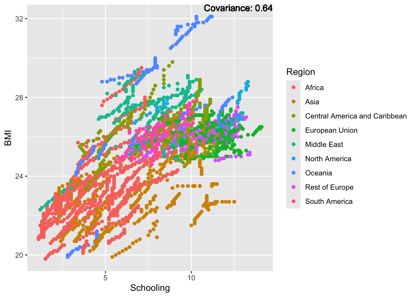

BMI Inferences:

Positive: Life Expectancy, Diphtheria, GDP, measles, polio, schooling

Negative: Thinness, infant deaths, under five deaths, adult mortality

Polio:

covariance_plot("Polio", "GDP_per_capita", df, sdf)

Warning in geom_text(aes(label = paste("Covariance:", round(cov(std_data_frame[[y_val]], : All aesthetics have length 1, but the data has 2864 rows.
ℹ Please consider using `annotate()` or provide this layer with data containing
  a single row.

covariance_plot("Polio", "Infant_deaths", df, sdf)

Warning in geom_text(aes(label = paste("Covariance:", round(cov(std_data_frame[[y_val]], : All aesthetics have length 1, but the data has 2864 rows.
ℹ Please consider using `annotate()` or provide this layer with data containing
  a single row.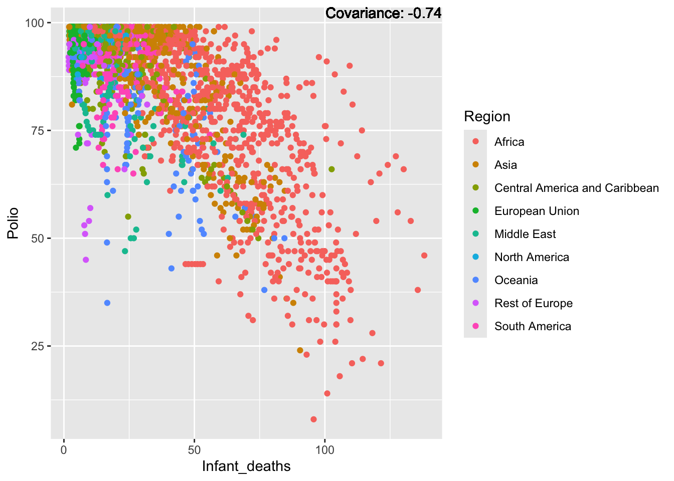

covariance_plot("Polio", "Under_five_deaths", df, sdf)

Warning in geom_text(aes(label = paste("Covariance:", round(cov(std_data_frame[[y_val]], : All aesthetics have length 1, but the data has 2864 rows.
ℹ Please consider using `annotate()` or provide this layer with data containing
  a single row.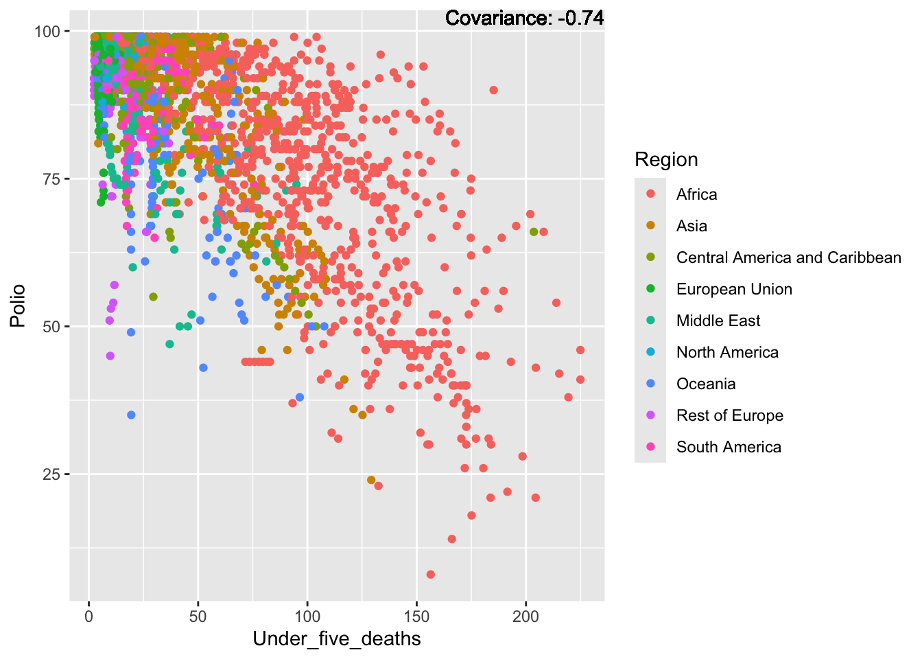

covariance_plot("Polio", "Life_expectancy", df, sdf)

Warning in geom_text(aes(label = paste("Covariance:", round(cov(std_data_frame[[y_val]], : All aesthetics have length 1, but the data has 2864 rows.
ℹ Please consider using `annotate()` or provide this layer with data containing
  a single row.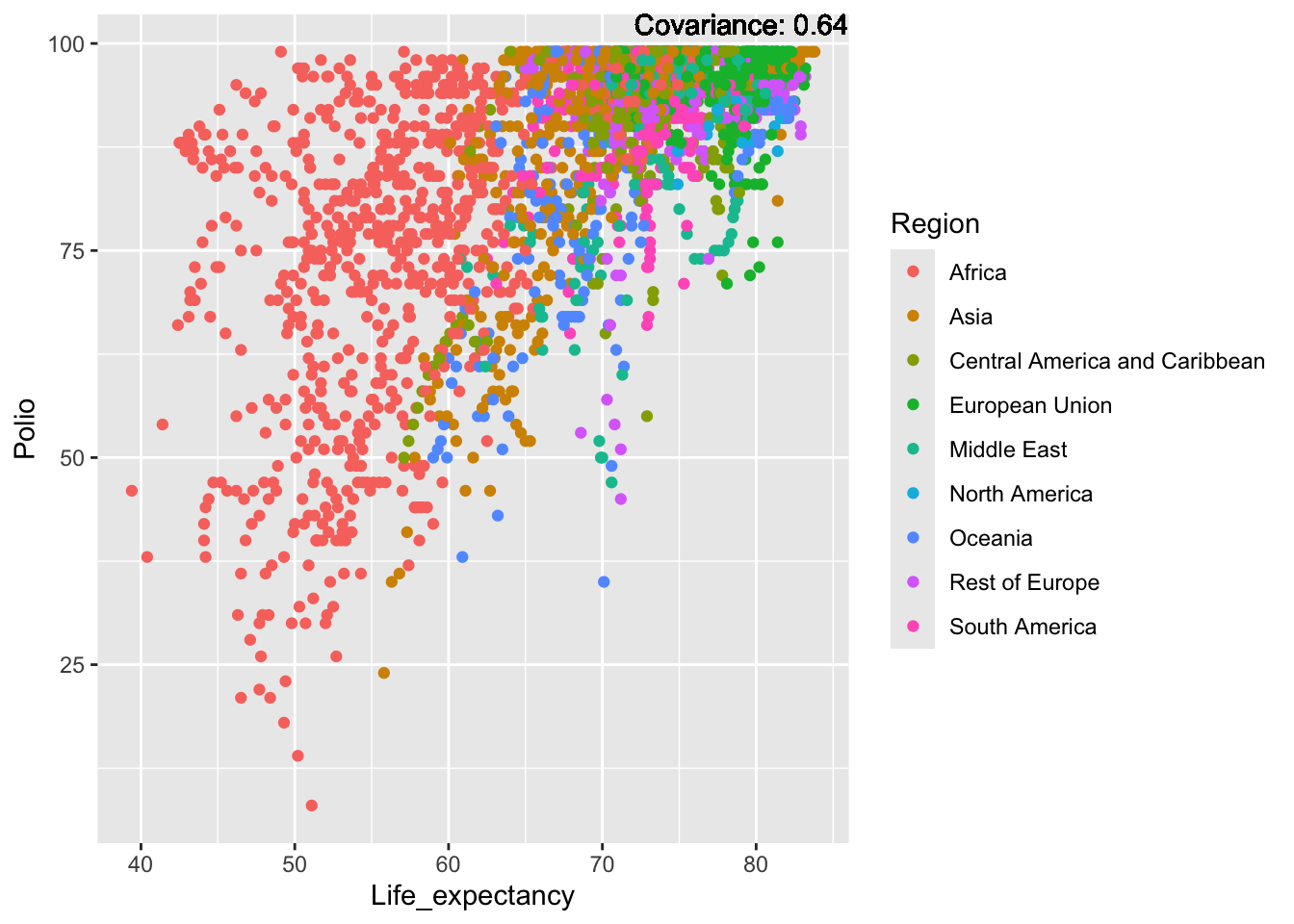

covariance_plot("Polio", "Adult_mortality", df, sdf)

Warning in geom_text(aes(label = paste("Covariance:", round(cov(std_data_frame[[y_val]], : All aesthetics have length 1, but the data has 2864 rows.
ℹ Please consider using `annotate()` or provide this layer with data containing
  a single row.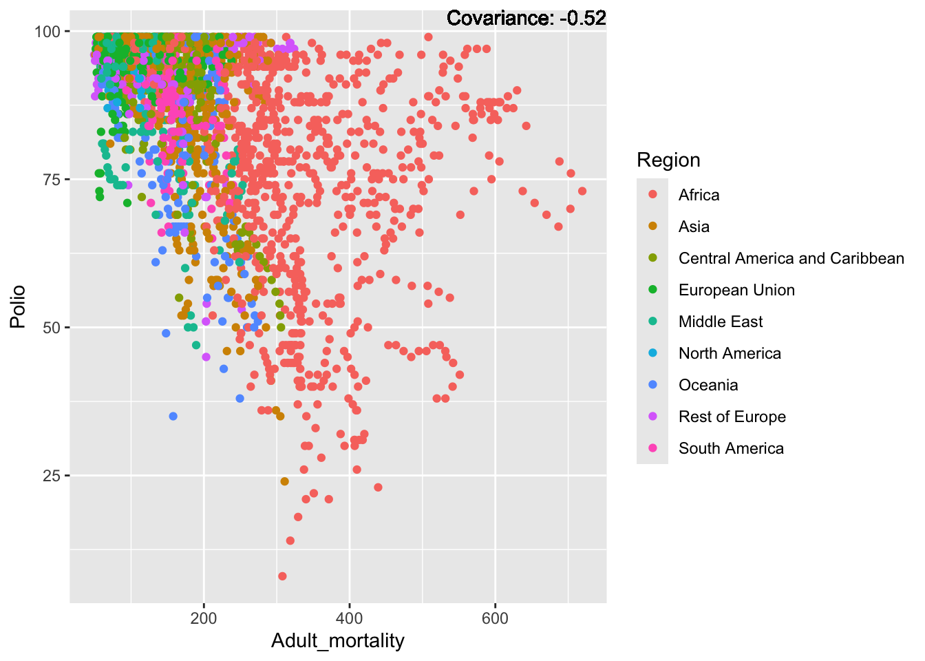

covariance_plot("Polio", "Hepatitis_B", df, sdf)

Warning in geom_text(aes(label = paste("Covariance:", round(cov(std_data_frame[[y_val]], : All aesthetics have length 1, but the data has 2864 rows.
ℹ Please consider using `annotate()` or provide this layer with data containing
  a single row.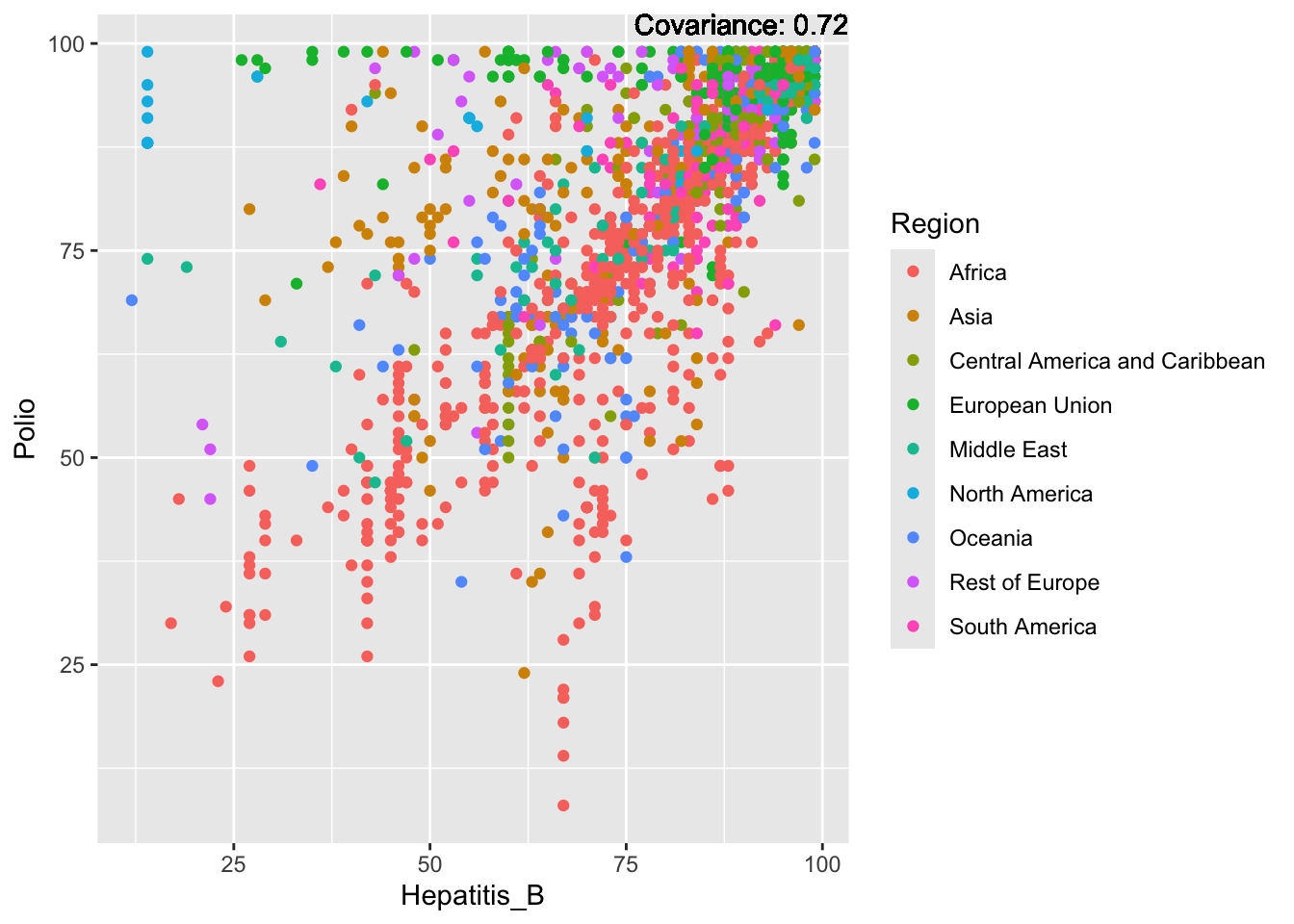

covariance_plot("Polio", "Measles", df, sdf)

Warning in geom_text(aes(label = paste("Covariance:", round(cov(std_data_frame[[y_val]], : All aesthetics have length 1, but the data has 2864 rows.
ℹ Please consider using `annotate()` or provide this layer with data containing
  a single row.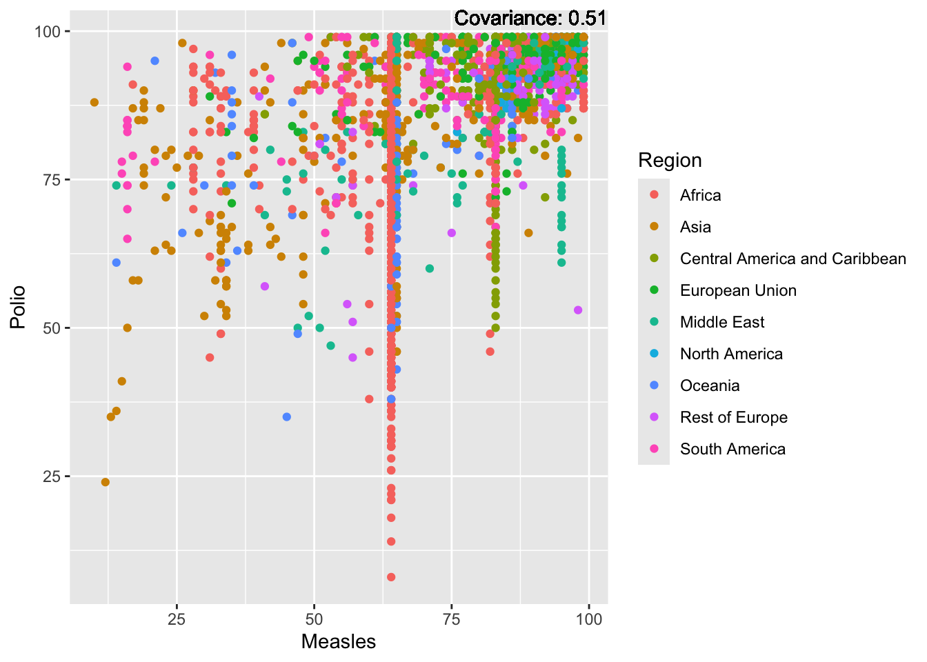

covariance_plot("Polio", "BMI", df, sdf)

Warning in geom_text(aes(label = paste("Covariance:", round(cov(std_data_frame[[y_val]], : All aesthetics have length 1, but the data has 2864 rows.
ℹ Please consider using `annotate()` or provide this layer with data containing
  a single row.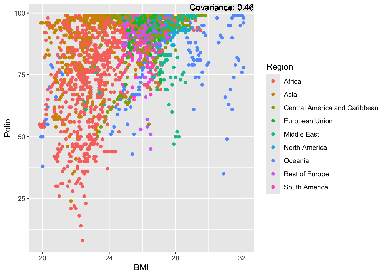

covariance_plot("Polio", "Diphtheria", df, sdf)

Warning in geom_text(aes(label = paste("Covariance:", round(cov(std_data_frame[[y_val]], : All aesthetics have length 1, but the data has 2864 rows.
ℹ Please consider using `annotate()` or provide this layer with data containing
  a single row.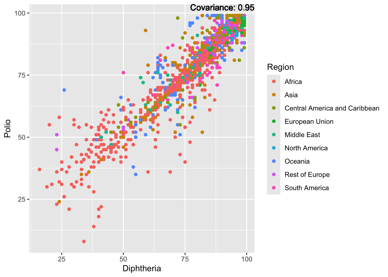

covariance_plot("Polio", "Incidents_HIV", df, sdf)

Warning in geom_text(aes(label = paste("Covariance:", round(cov(std_data_frame[[y_val]], : All aesthetics have length 1, but the data has 2864 rows.
ℹ Please consider using `annotate()` or provide this layer with data containing
  a single row.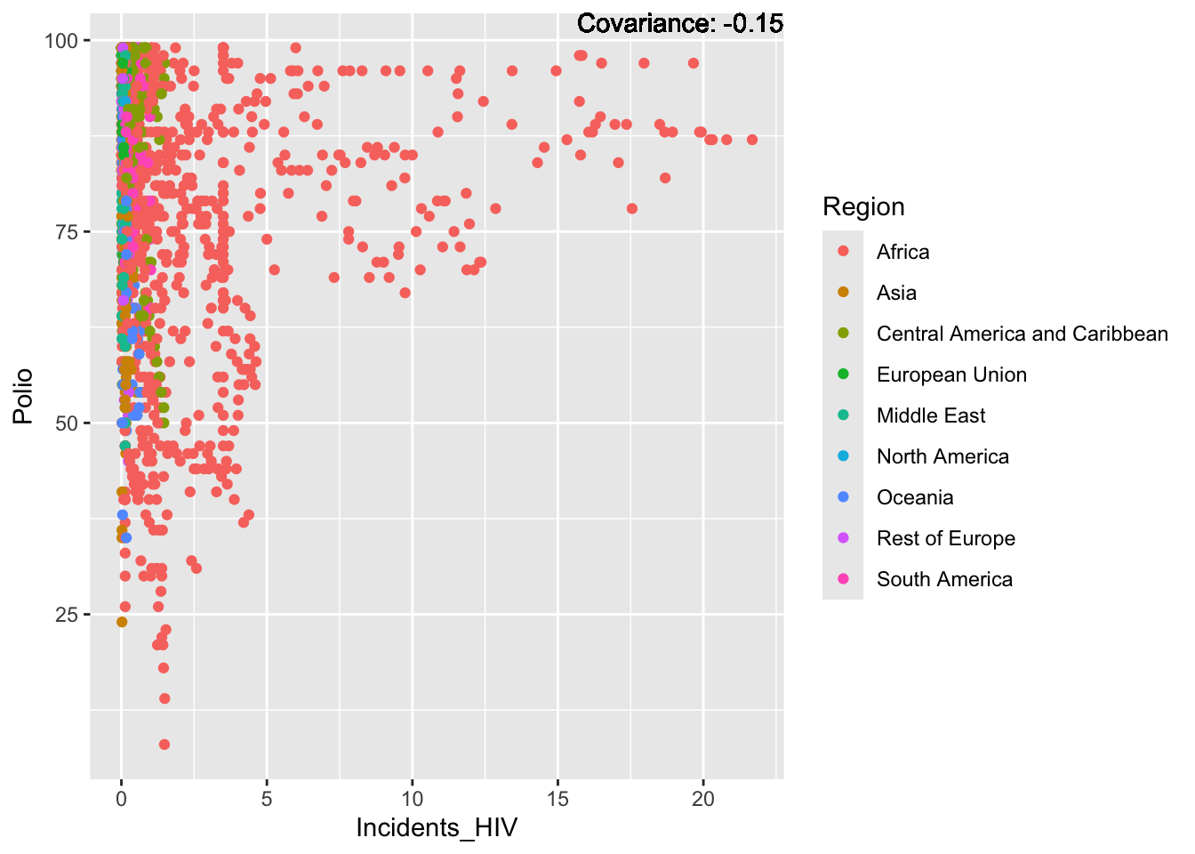

covariance_plot("Polio", "Alcohol_consumption", df, sdf)

Warning in geom_text(aes(label = paste("Covariance:", round(cov(std_data_frame[[y_val]], : All aesthetics have length 1, but the data has 2864 rows.
ℹ Please consider using `annotate()` or provide this layer with data containing
  a single row.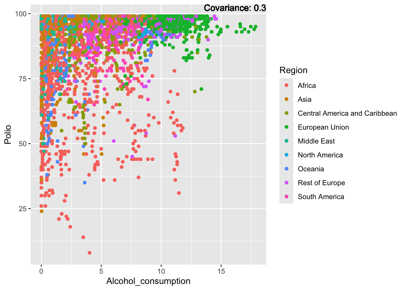

covariance_plot("Polio", "Population_mln", df, sdf)

Warning in geom_text(aes(label = paste("Covariance:", round(cov(std_data_frame[[y_val]], : All aesthetics have length 1, but the data has 2864 rows.
ℹ Please consider using `annotate()` or provide this layer with data containing
  a single row.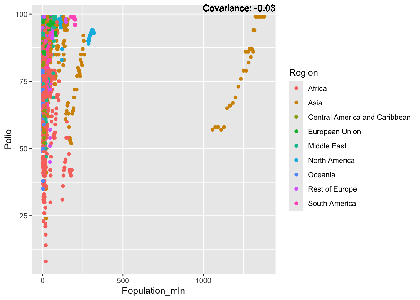

covariance_plot("Polio", "Thinness_ten_nineteen_years", df, sdf)

Warning in geom_text(aes(label = paste("Covariance:", round(cov(std_data_frame[[y_val]], : All aesthetics have length 1, but the data has 2864 rows.
ℹ Please consider using `annotate()` or provide this layer with data containing
  a single row.

covariance_plot("Polio", "Thinness_five_nine_years", df, sdf)

Warning in geom_text(aes(label = paste("Covariance:", round(cov(std_data_frame[[y_val]], : All aesthetics have length 1, but the data has 2864 rows.
ℹ Please consider using `annotate()` or provide this layer with data containing
  a single row.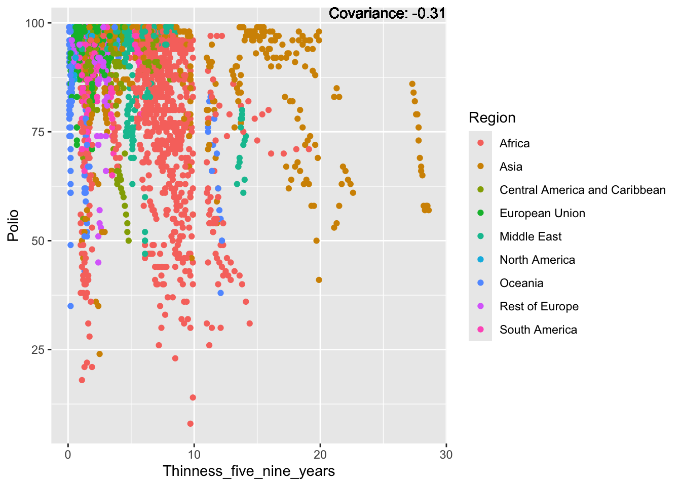

covariance_plot("Polio", "Schooling", df, sdf)

Warning in geom_text(aes(label = paste("Covariance:", round(cov(std_data_frame[[y_val]], : All aesthetics have length 1, but the data has 2864 rows.
ℹ Please consider using `annotate()` or provide this layer with data containing
  a single row.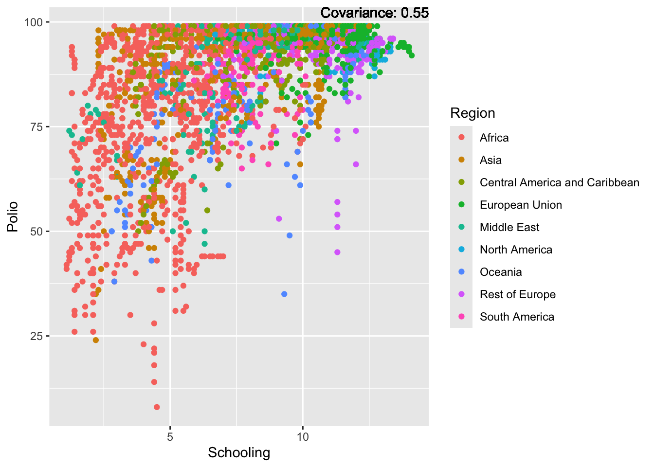

Polio Inferences:

Strong Positive, Hepatitis B, Diphtheria

Positive: Polio, BMI, Schooling, life expectancy, measles

Negative: Thinness, adult mortality

Strong Negative: Infant Deaths, Under Five deaths

Diphtheria:

covariance_plot("Diphtheria", "GDP_per_capita", df, sdf)

Warning in geom_text(aes(label = paste("Covariance:", round(cov(std_data_frame[[y_val]], : All aesthetics have length 1, but the data has 2864 rows.
ℹ Please consider using `annotate()` or provide this layer with data containing
  a single row.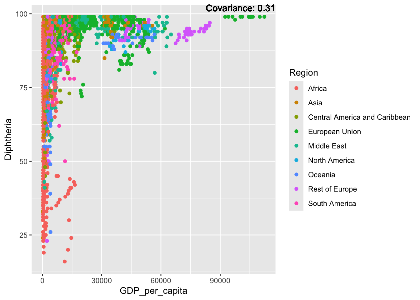

covariance_plot("Diphtheria", "Infant_deaths", df, sdf)

Warning in geom_text(aes(label = paste("Covariance:", round(cov(std_data_frame[[y_val]], : All aesthetics have length 1, but the data has 2864 rows.
ℹ Please consider using `annotate()` or provide this layer with data containing
  a single row.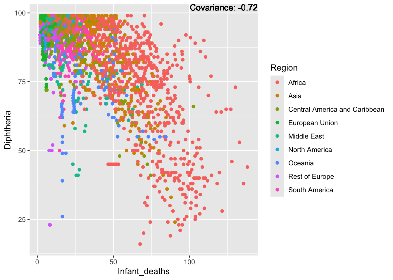

covariance_plot("Diphtheria", "Under_five_deaths", df, sdf)

Warning in geom_text(aes(label = paste("Covariance:", round(cov(std_data_frame[[y_val]], : All aesthetics have length 1, but the data has 2864 rows.
ℹ Please consider using `annotate()` or provide this layer with data containing
  a single row.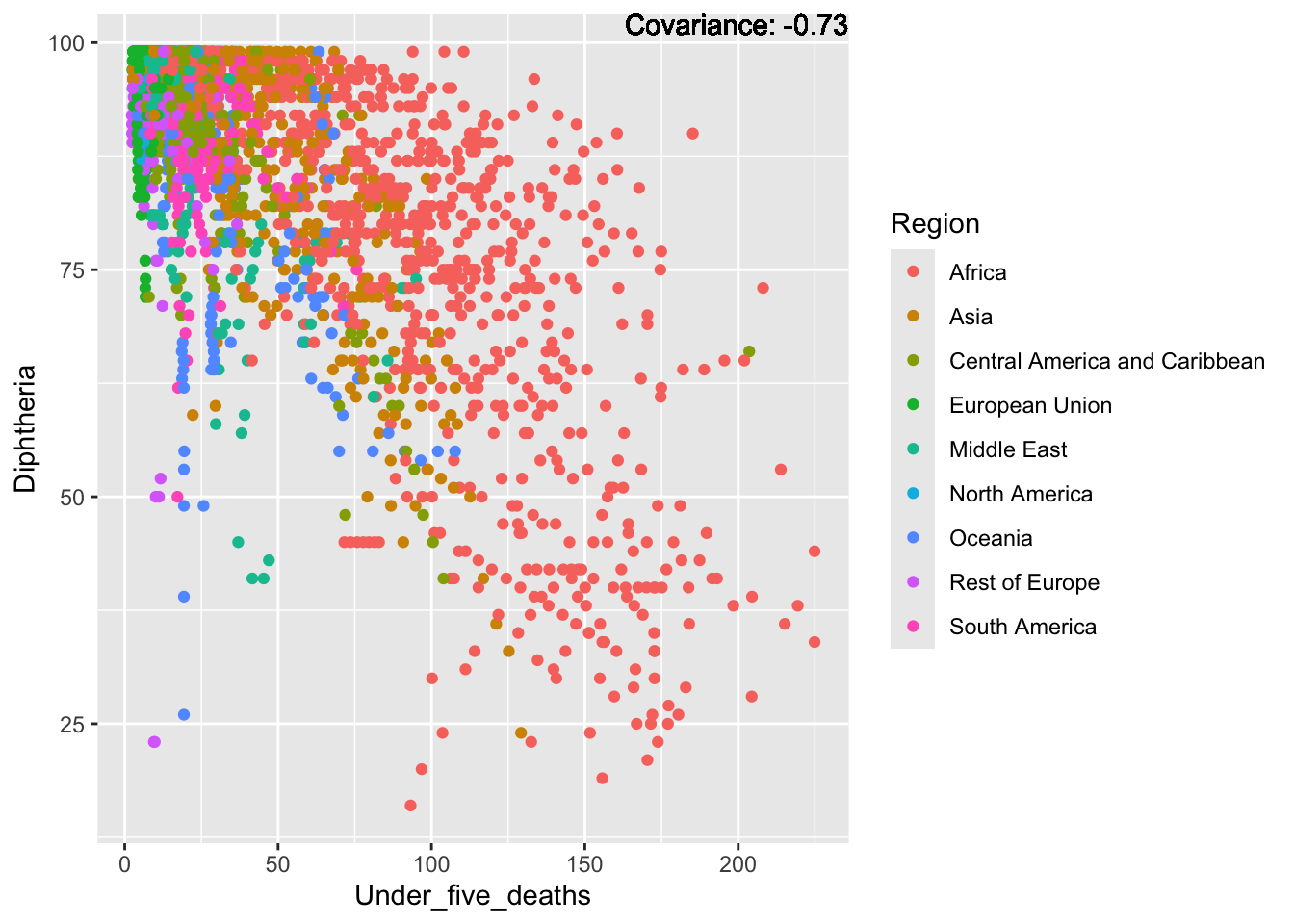

covariance_plot("Diphtheria", "Life_expectancy", df, sdf)

Warning in geom_text(aes(label = paste("Covariance:", round(cov(std_data_frame[[y_val]], : All aesthetics have length 1, but the data has 2864 rows.
ℹ Please consider using `annotate()` or provide this layer with data containing
  a single row.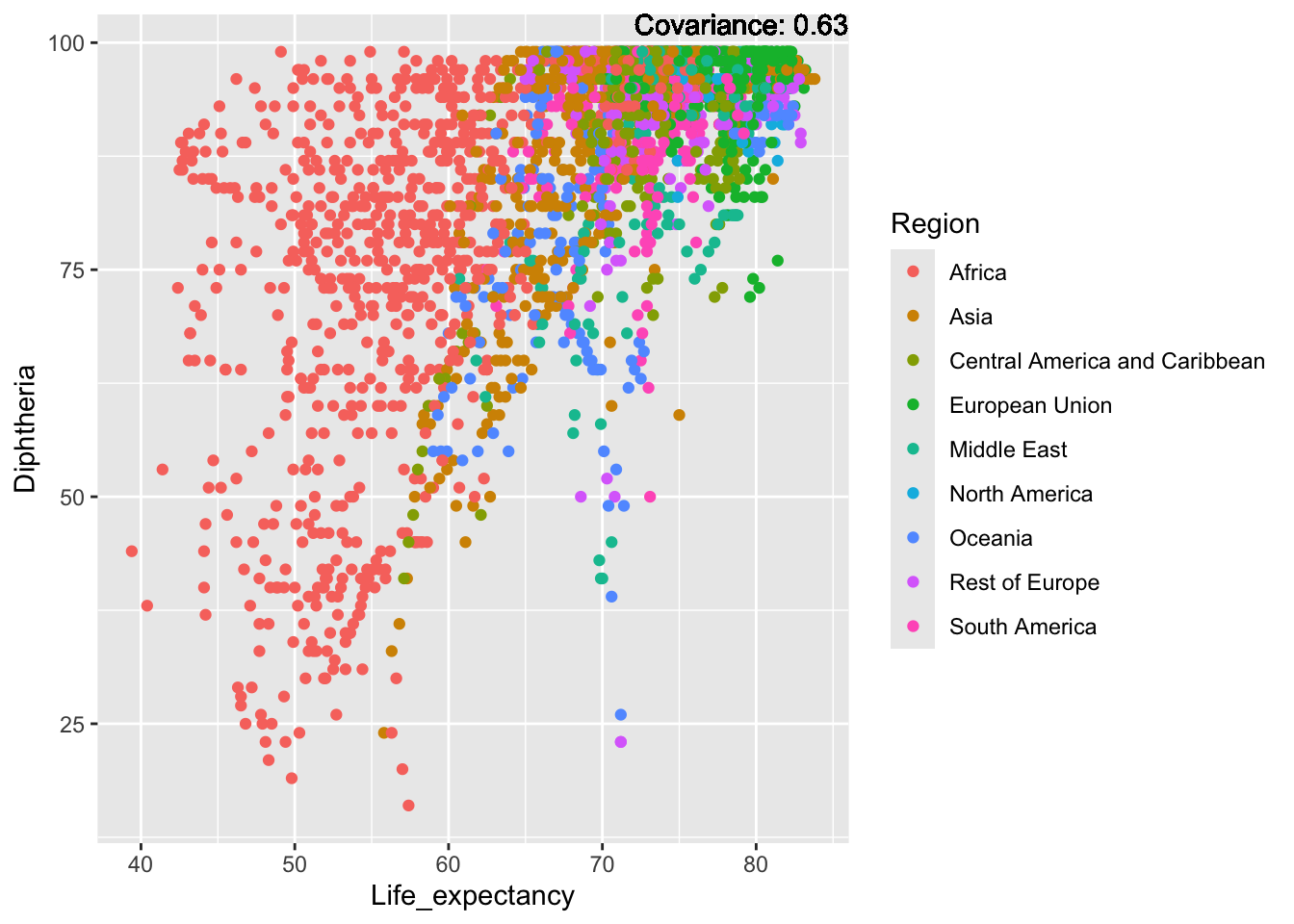

covariance_plot("Diphtheria", "Adult_mortality", df, sdf)

Warning in geom_text(aes(label = paste("Covariance:", round(cov(std_data_frame[[y_val]], : All aesthetics have length 1, but the data has 2864 rows.
ℹ Please consider using `annotate()` or provide this layer with data containing
  a single row.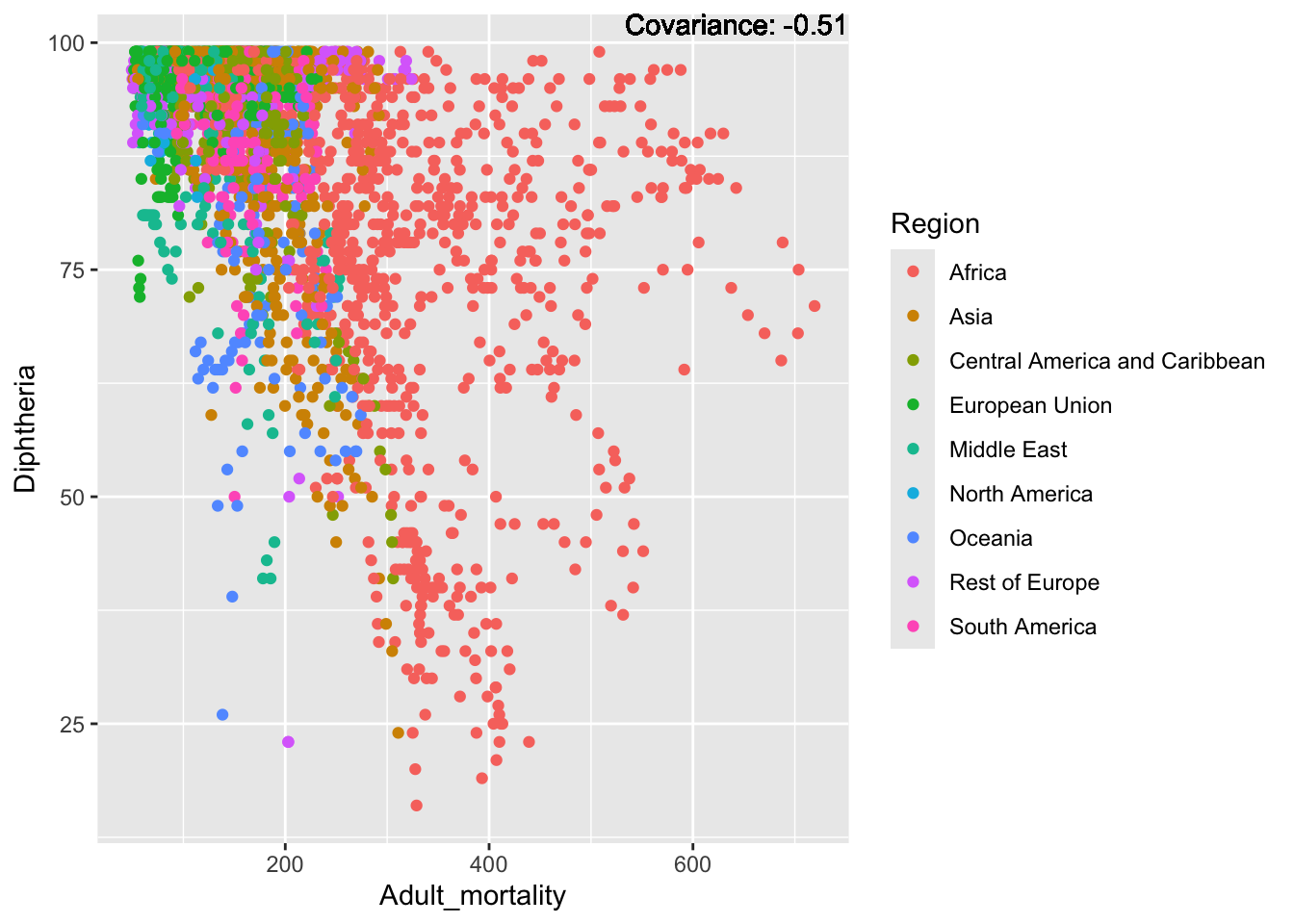

covariance_plot("Diphtheria", "Hepatitis_B", df, sdf)

Warning in geom_text(aes(label = paste("Covariance:", round(cov(std_data_frame[[y_val]], : All aesthetics have length 1, but the data has 2864 rows.
ℹ Please consider using `annotate()` or provide this layer with data containing
  a single row.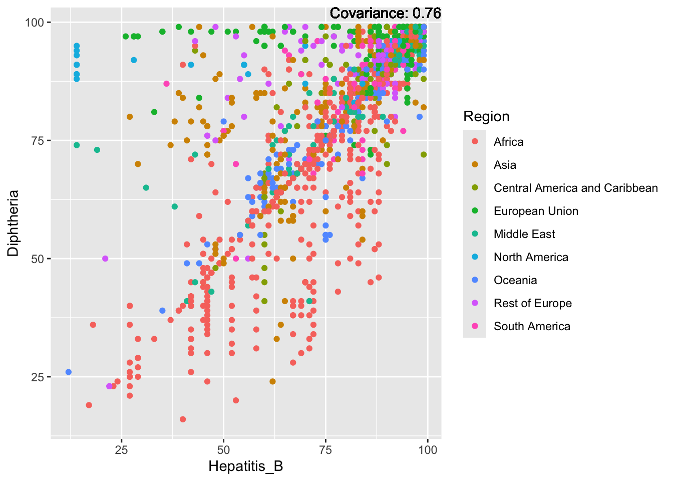

covariance_plot("Diphtheria", "Measles", df, sdf)

Warning in geom_text(aes(label = paste("Covariance:", round(cov(std_data_frame[[y_val]], : All aesthetics have length 1, but the data has 2864 rows.
ℹ Please consider using `annotate()` or provide this layer with data containing
  a single row.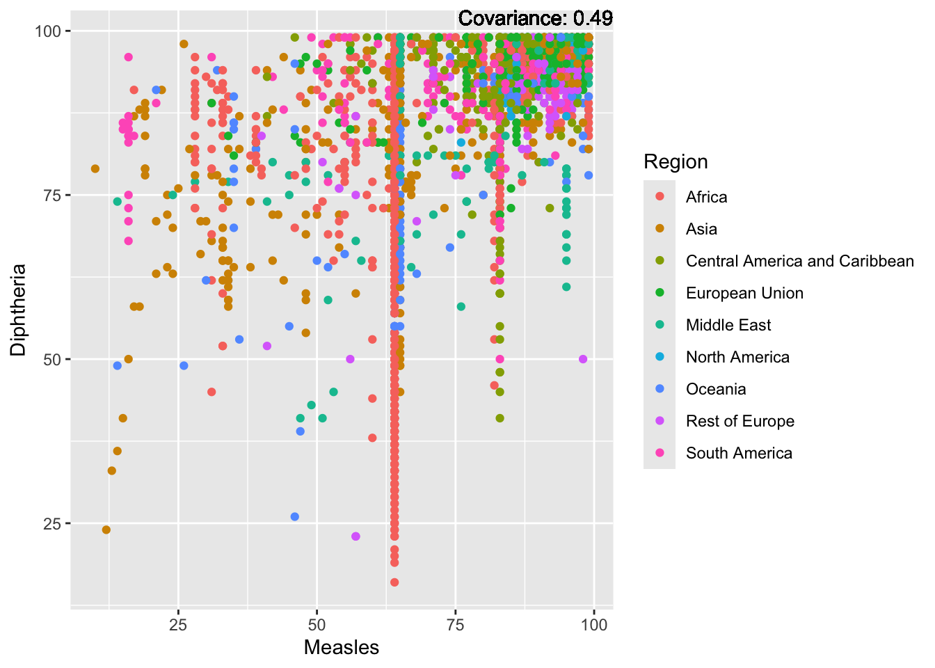

covariance_plot("Diphtheria", "BMI", df, sdf)

Warning in geom_text(aes(label = paste("Covariance:", round(cov(std_data_frame[[y_val]], : All aesthetics have length 1, but the data has 2864 rows.
ℹ Please consider using `annotate()` or provide this layer with data containing
  a single row.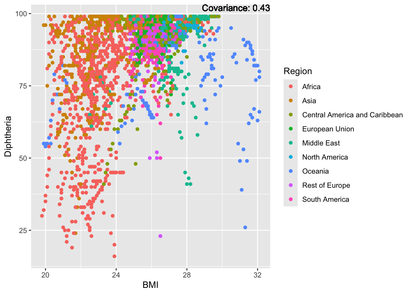

covariance_plot("Diphtheria", "Polio", df, sdf)

Warning in geom_text(aes(label = paste("Covariance:", round(cov(std_data_frame[[y_val]], : All aesthetics have length 1, but the data has 2864 rows.
ℹ Please consider using `annotate()` or provide this layer with data containing
  a single row.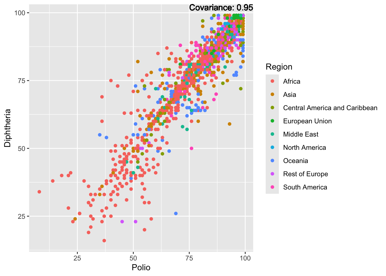

covariance_plot("Diphtheria", "Incidents_HIV", df, sdf)

Warning in geom_text(aes(label = paste("Covariance:", round(cov(std_data_frame[[y_val]], : All aesthetics have length 1, but the data has 2864 rows.
ℹ Please consider using `annotate()` or provide this layer with data containing
  a single row.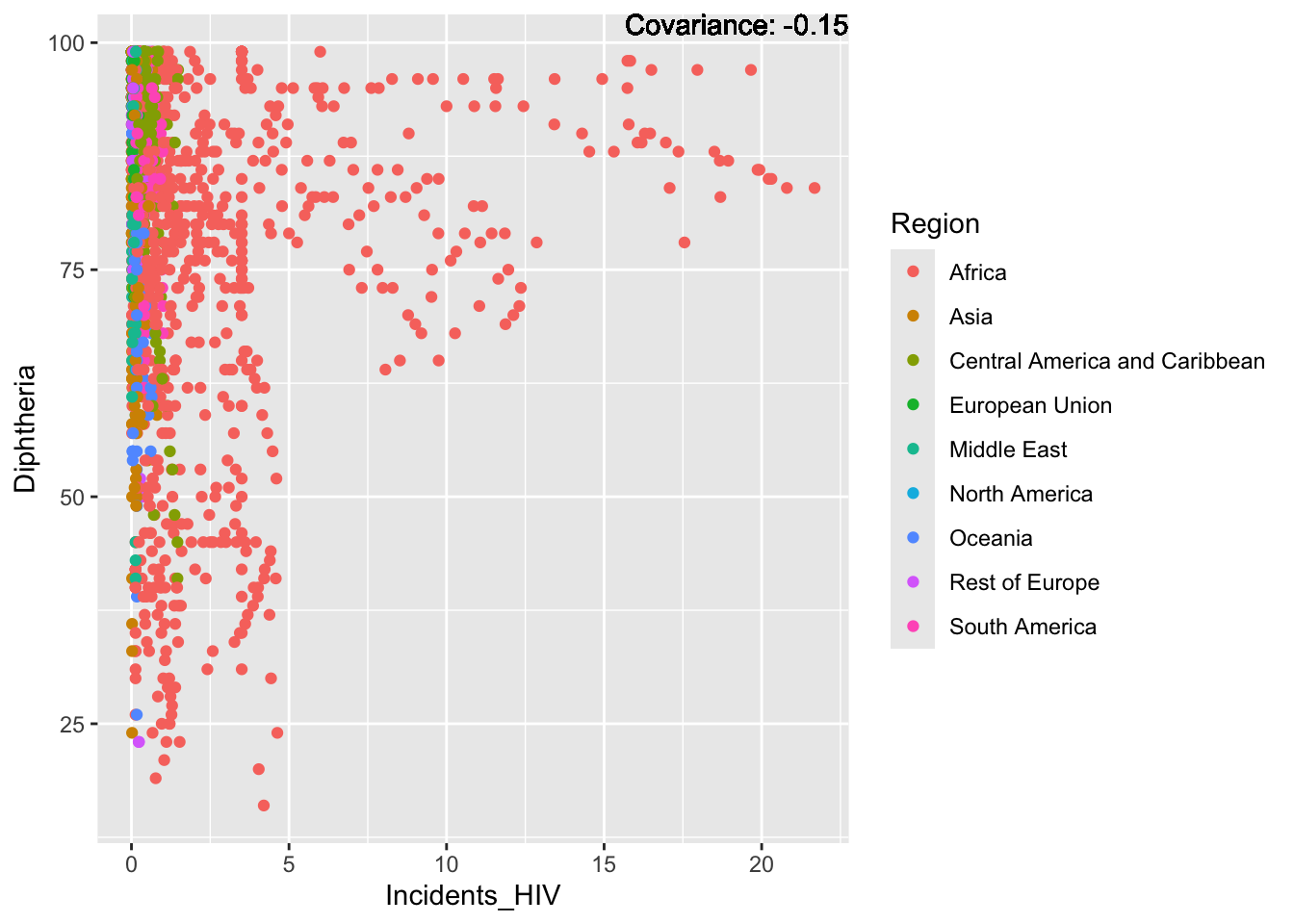

covariance_plot("Diphtheria", "Alcohol_consumption", df, sdf)

Warning in geom_text(aes(label = paste("Covariance:", round(cov(std_data_frame[[y_val]], : All aesthetics have length 1, but the data has 2864 rows.
ℹ Please consider using `annotate()` or provide this layer with data containing
  a single row.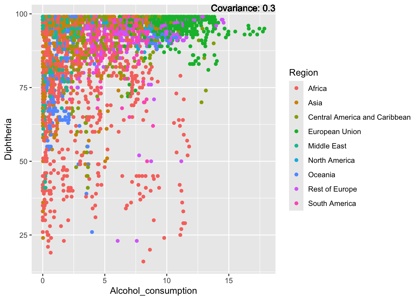

covariance_plot("Diphtheria", "Population_mln", df, sdf)

Warning in geom_text(aes(label = paste("Covariance:", round(cov(std_data_frame[[y_val]], : All aesthetics have length 1, but the data has 2864 rows.
ℹ Please consider using `annotate()` or provide this layer with data containing
  a single row.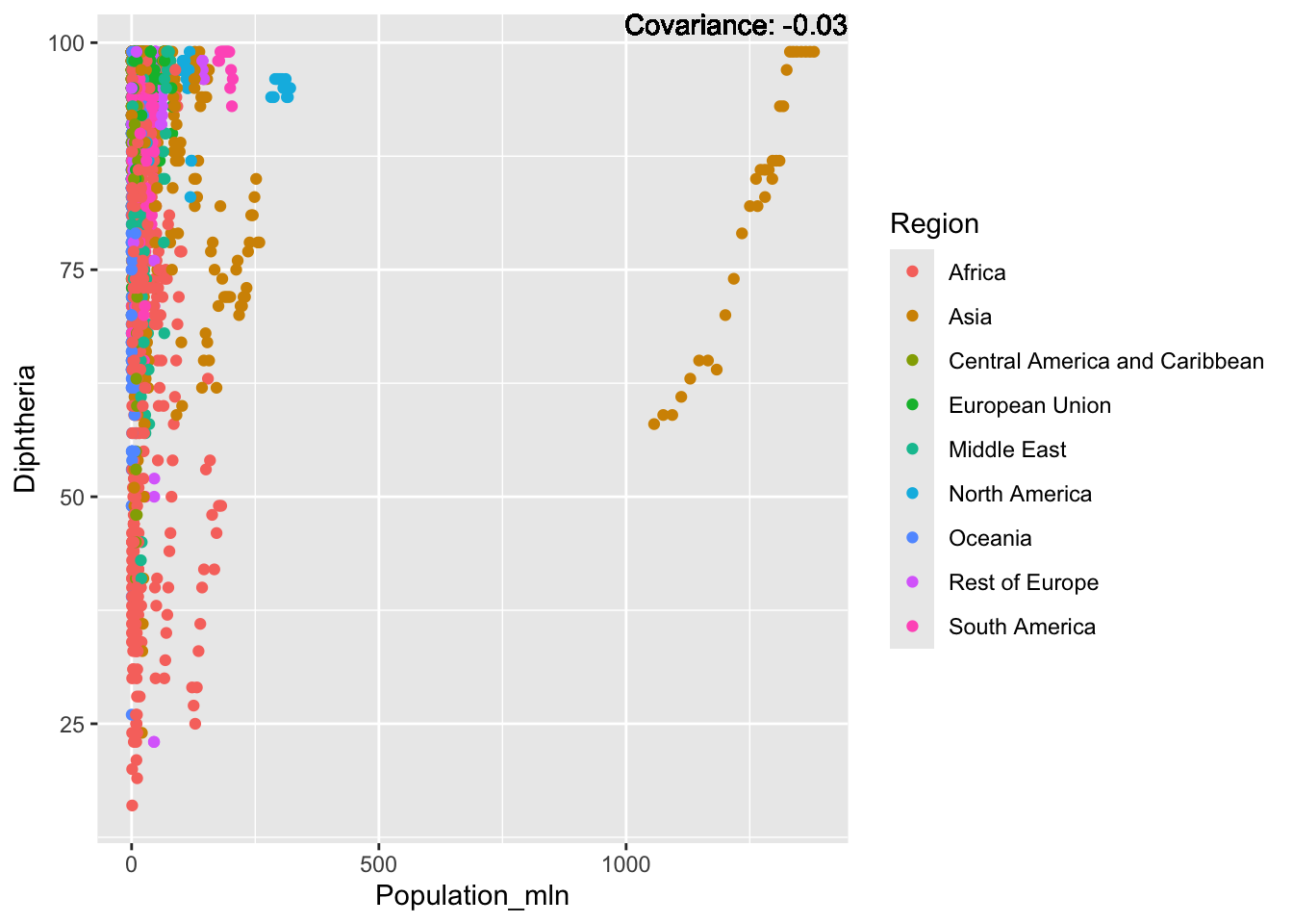

covariance_plot("Diphtheria", "Thinness_ten_nineteen_years", df, sdf)

Warning in geom_text(aes(label = paste("Covariance:", round(cov(std_data_frame[[y_val]], : All aesthetics have length 1, but the data has 2864 rows.
ℹ Please consider using `annotate()` or provide this layer with data containing
  a single row.

covariance_plot("Diphtheria", "Thinness_five_nine_years", df, sdf)

Warning in geom_text(aes(label = paste("Covariance:", round(cov(std_data_frame[[y_val]], : All aesthetics have length 1, but the data has 2864 rows.
ℹ Please consider using `annotate()` or provide this layer with data containing
  a single row.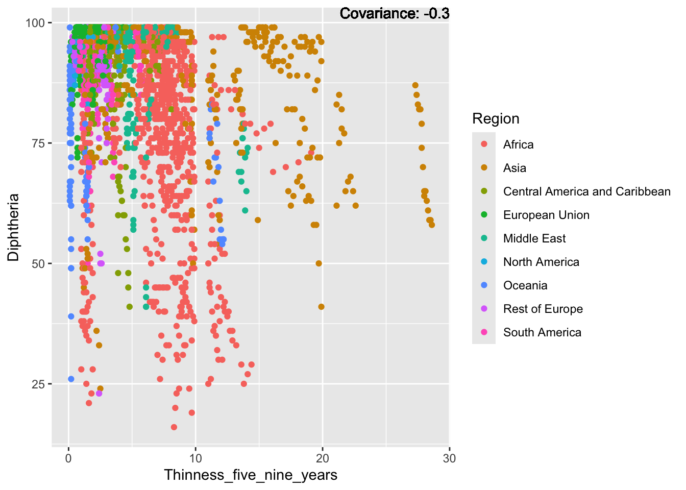

covariance_plot("Diphtheria", "Schooling", df, sdf)

Warning in geom_text(aes(label = paste("Covariance:", round(cov(std_data_frame[[y_val]], : All aesthetics have length 1, but the data has 2864 rows.
ℹ Please consider using `annotate()` or provide this layer with data containing
  a single row.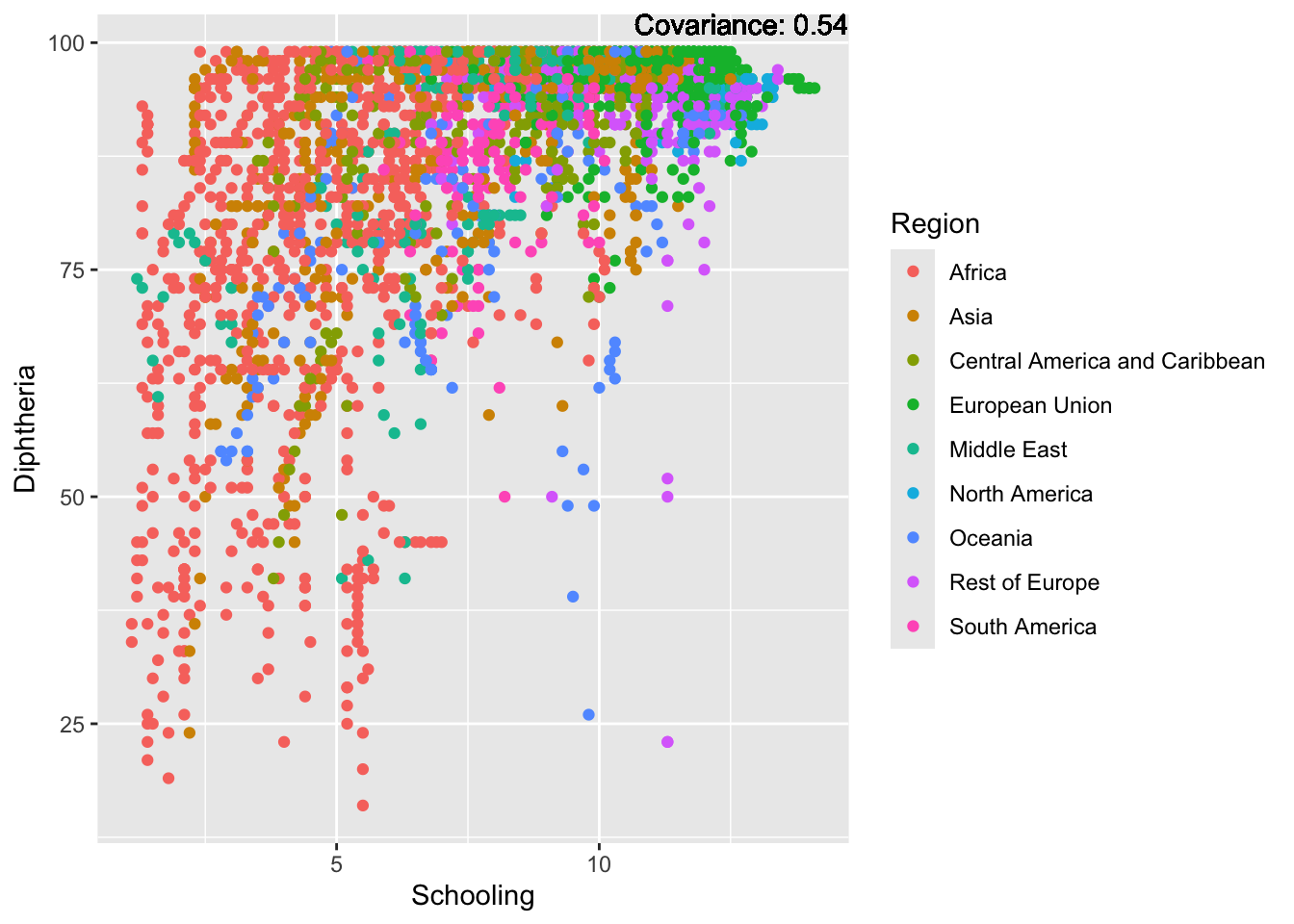

Diphtheria Inferences:

Strong Positive: Hepatitis B, Polio

Positive: Life Expectancy, Measles, BMI, Schooling

Negative: Thinness, adult mortality

Strong Negative: Infant Deaths, Under Five Deaths

HIV:

covariance_plot("Incidents_HIV", "GDP_per_capita", df, sdf)

Warning in geom_text(aes(label = paste("Covariance:", round(cov(std_data_frame[[y_val]], : All aesthetics have length 1, but the data has 2864 rows.
ℹ Please consider using `annotate()` or provide this layer with data containing
  a single row.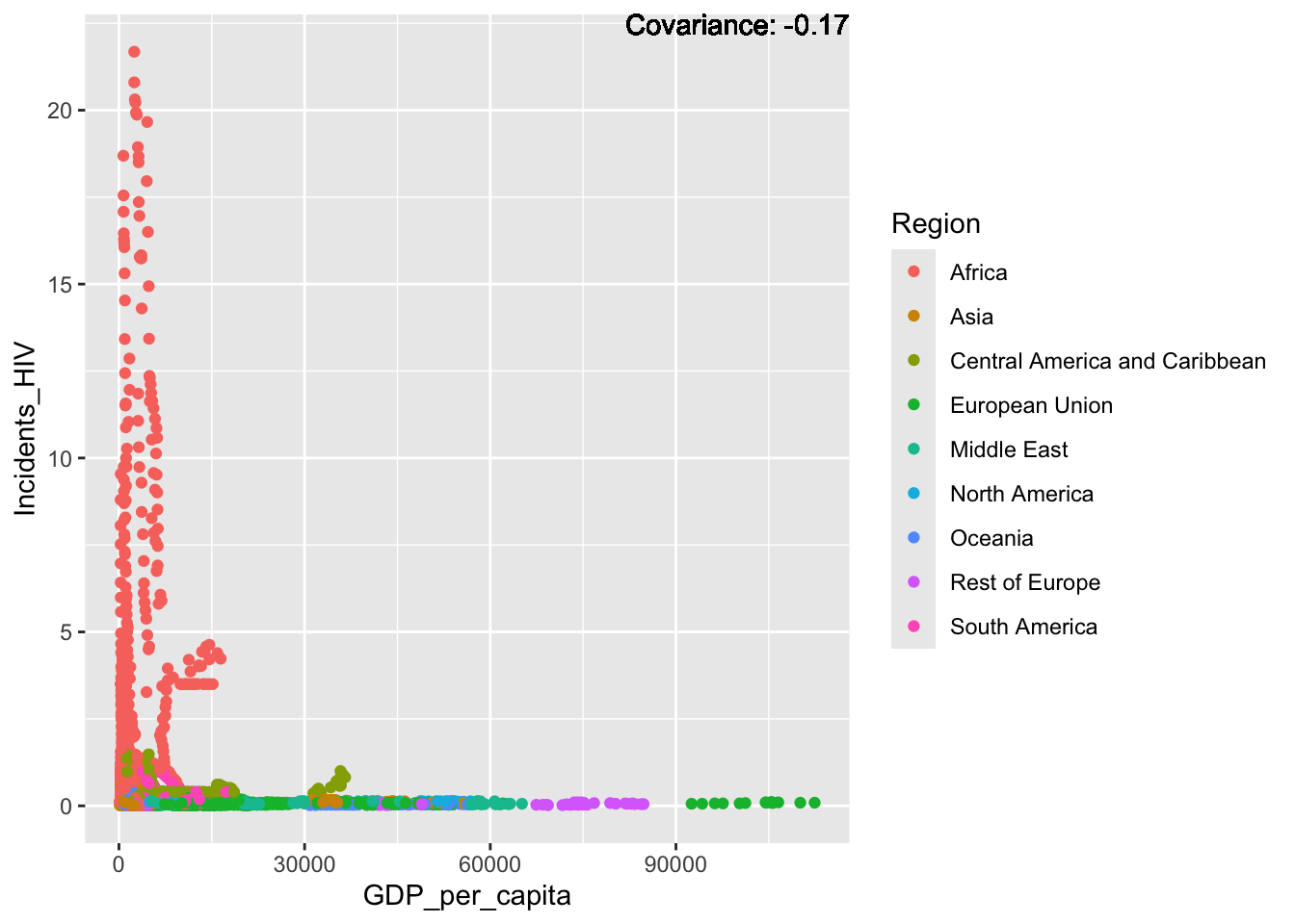

covariance_plot("Incidents_HIV", "Infant_deaths", df, sdf)

Warning in geom_text(aes(label = paste("Covariance:", round(cov(std_data_frame[[y_val]], : All aesthetics have length 1, but the data has 2864 rows.
ℹ Please consider using `annotate()` or provide this layer with data containing
  a single row.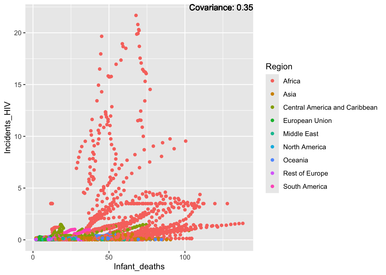

covariance_plot("Incidents_HIV", "Under_five_deaths", df, sdf)

Warning in geom_text(aes(label = paste("Covariance:", round(cov(std_data_frame[[y_val]], : All aesthetics have length 1, but the data has 2864 rows.
ℹ Please consider using `annotate()` or provide this layer with data containing
  a single row.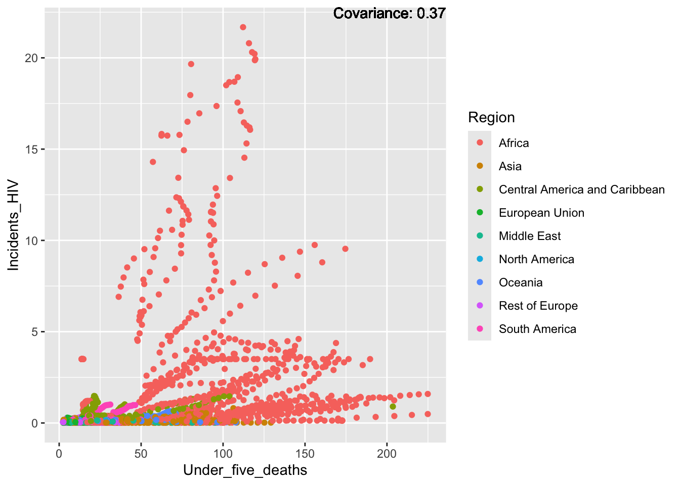

covariance_plot("Incidents_HIV", "Life_expectancy", df, sdf)

Warning in geom_text(aes(label = paste("Covariance:", round(cov(std_data_frame[[y_val]], : All aesthetics have length 1, but the data has 2864 rows.
ℹ Please consider using `annotate()` or provide this layer with data containing
  a single row.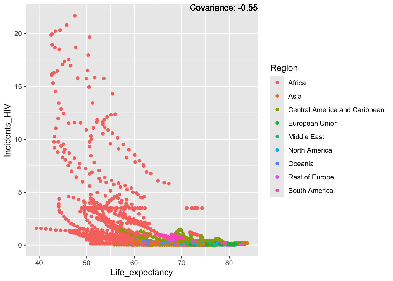

covariance_plot("Incidents_HIV", "Adult_mortality", df, sdf)

Warning in geom_text(aes(label = paste("Covariance:", round(cov(std_data_frame[[y_val]], : All aesthetics have length 1, but the data has 2864 rows.
ℹ Please consider using `annotate()` or provide this layer with data containing
  a single row.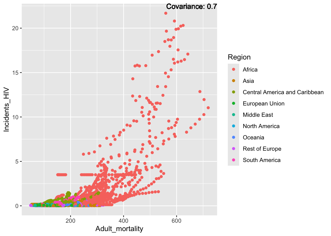

covariance_plot("Incidents_HIV", "Hepatitis_B", df, sdf)

Warning in geom_text(aes(label = paste("Covariance:", round(cov(std_data_frame[[y_val]], : All aesthetics have length 1, but the data has 2864 rows.
ℹ Please consider using `annotate()` or provide this layer with data containing
  a single row.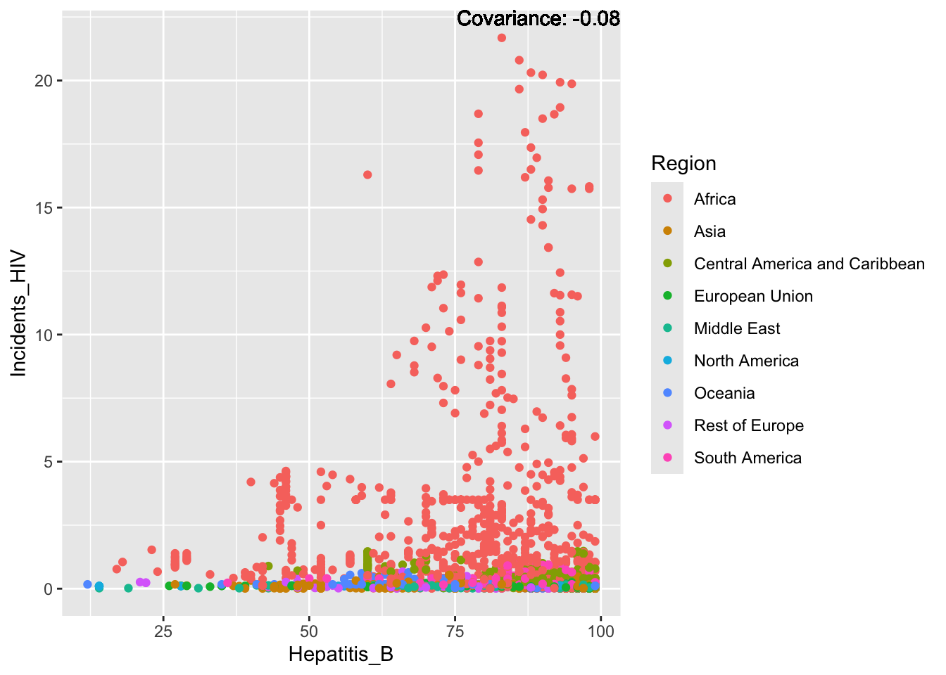

covariance_plot("Incidents_HIV", "Measles", df, sdf)

Warning in geom_text(aes(label = paste("Covariance:", round(cov(std_data_frame[[y_val]], : All aesthetics have length 1, but the data has 2864 rows.
ℹ Please consider using `annotate()` or provide this layer with data containing
  a single row.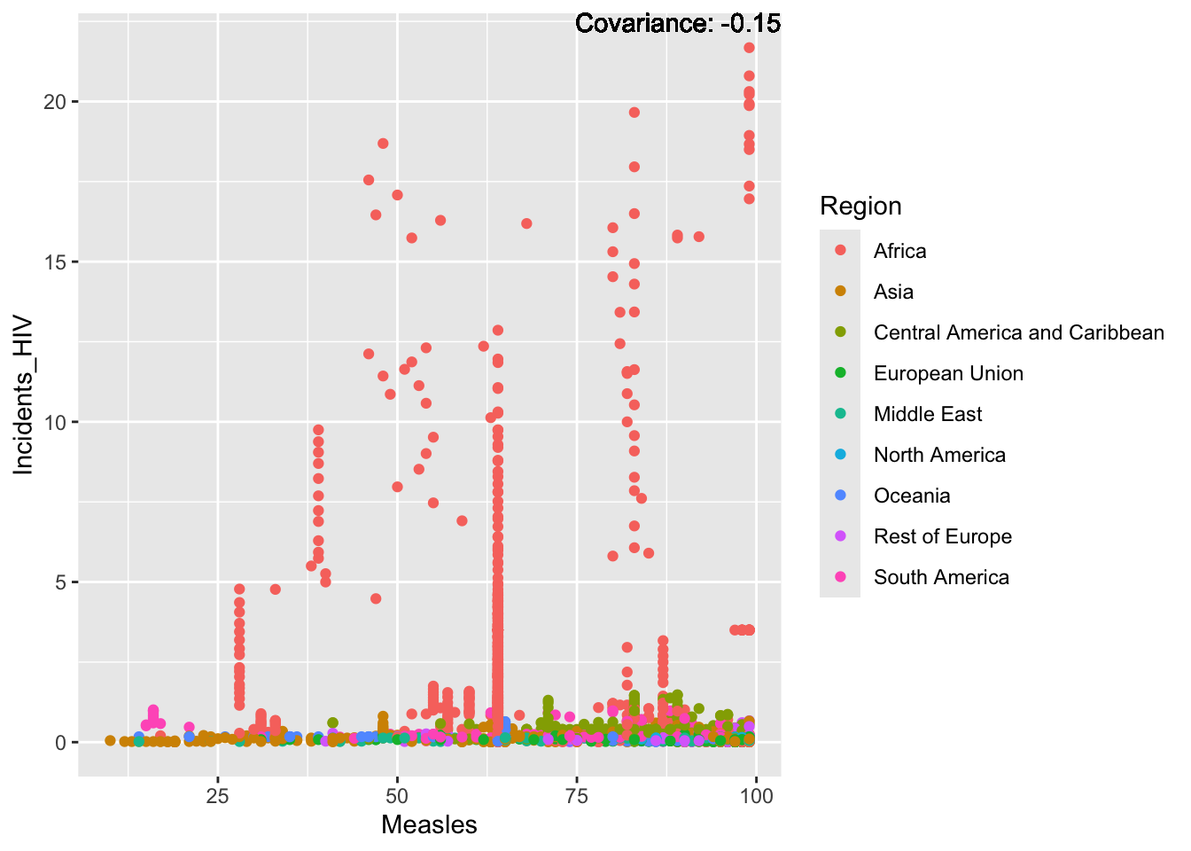

covariance_plot("Incidents_HIV", "BMI", df, sdf)

Warning in geom_text(aes(label = paste("Covariance:", round(cov(std_data_frame[[y_val]], : All aesthetics have length 1, but the data has 2864 rows.
ℹ Please consider using `annotate()` or provide this layer with data containing
  a single row.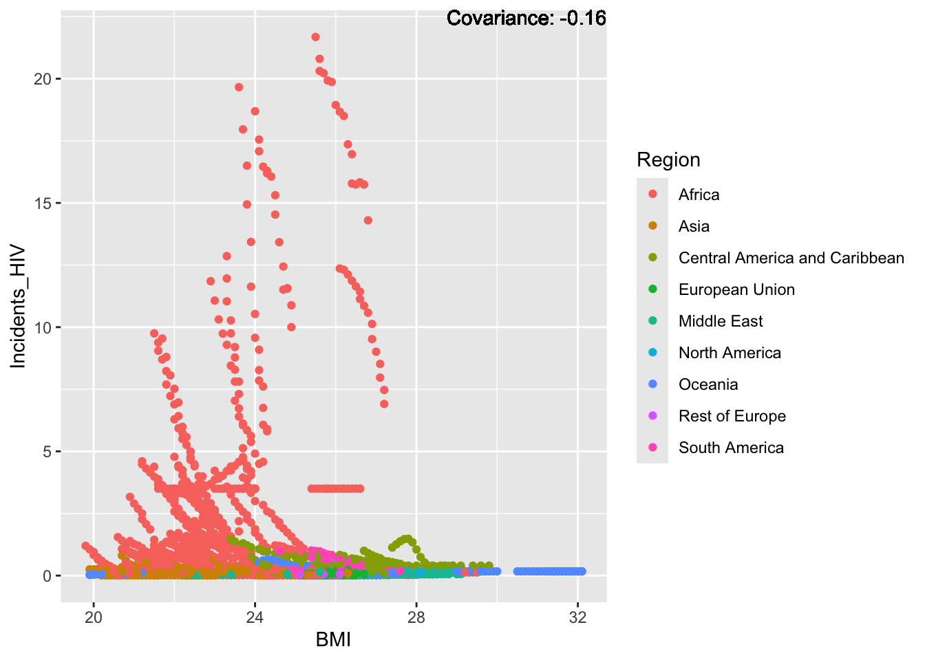

covariance_plot("Incidents_HIV", "Polio", df, sdf)

Warning in geom_text(aes(label = paste("Covariance:", round(cov(std_data_frame[[y_val]], : All aesthetics have length 1, but the data has 2864 rows.
ℹ Please consider using `annotate()` or provide this layer with data containing
  a single row.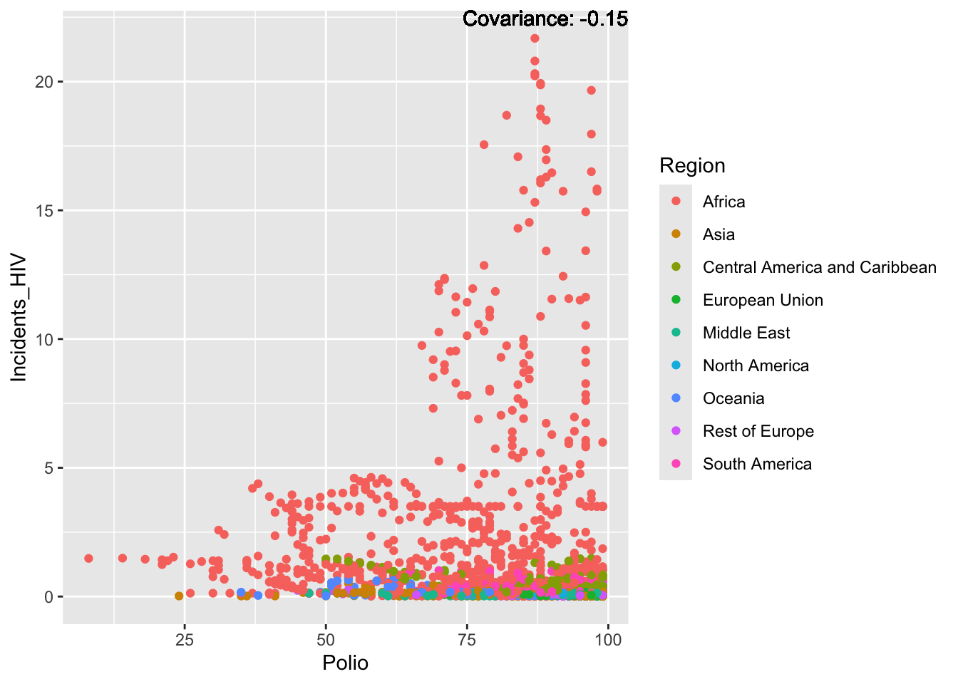

covariance_plot("Incidents_HIV", "Diphtheria", df, sdf)

Warning in geom_text(aes(label = paste("Covariance:", round(cov(std_data_frame[[y_val]], : All aesthetics have length 1, but the data has 2864 rows.
ℹ Please consider using `annotate()` or provide this layer with data containing
  a single row.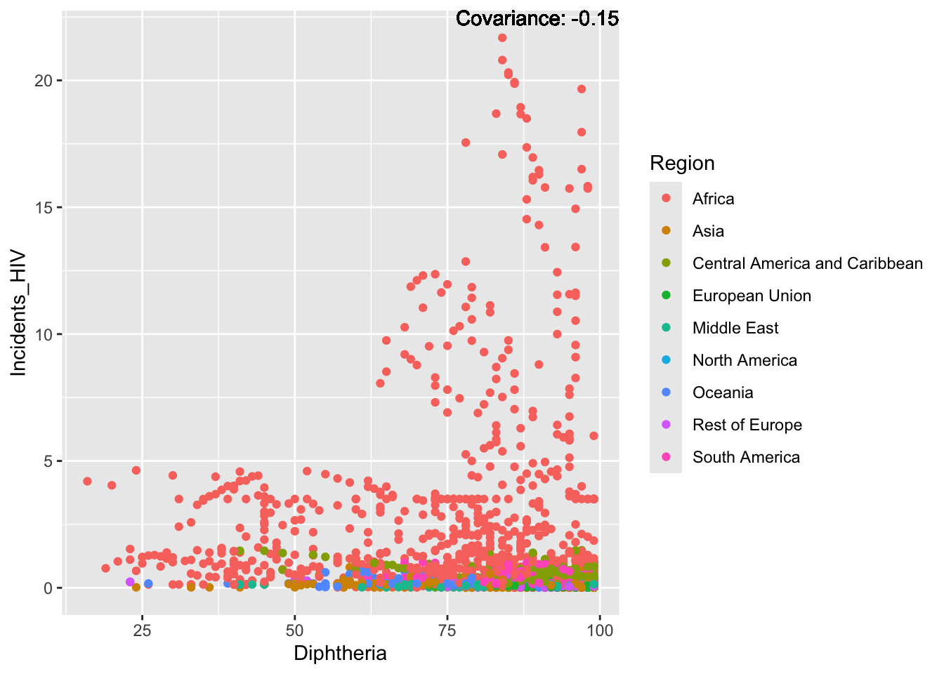

covariance_plot("Incidents_HIV", "Alcohol_consumption", df, sdf)

Warning in geom_text(aes(label = paste("Covariance:", round(cov(std_data_frame[[y_val]], : All aesthetics have length 1, but the data has 2864 rows.
ℹ Please consider using `annotate()` or provide this layer with data containing
  a single row.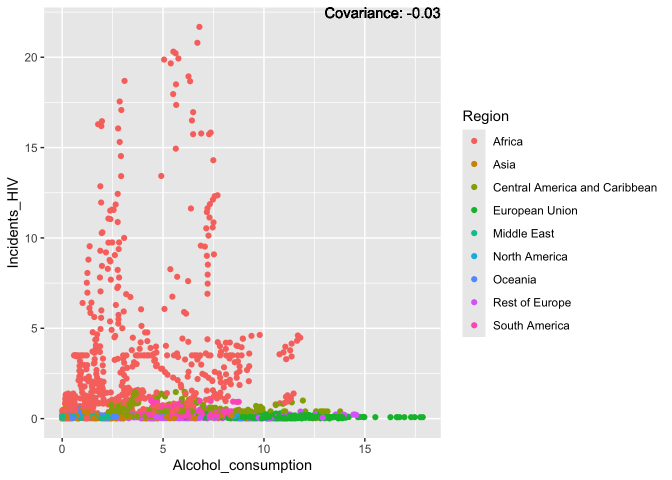

covariance_plot("Incidents_HIV", "Population_mln", df, sdf)

Warning in geom_text(aes(label = paste("Covariance:", round(cov(std_data_frame[[y_val]], : All aesthetics have length 1, but the data has 2864 rows.
ℹ Please consider using `annotate()` or provide this layer with data containing
  a single row.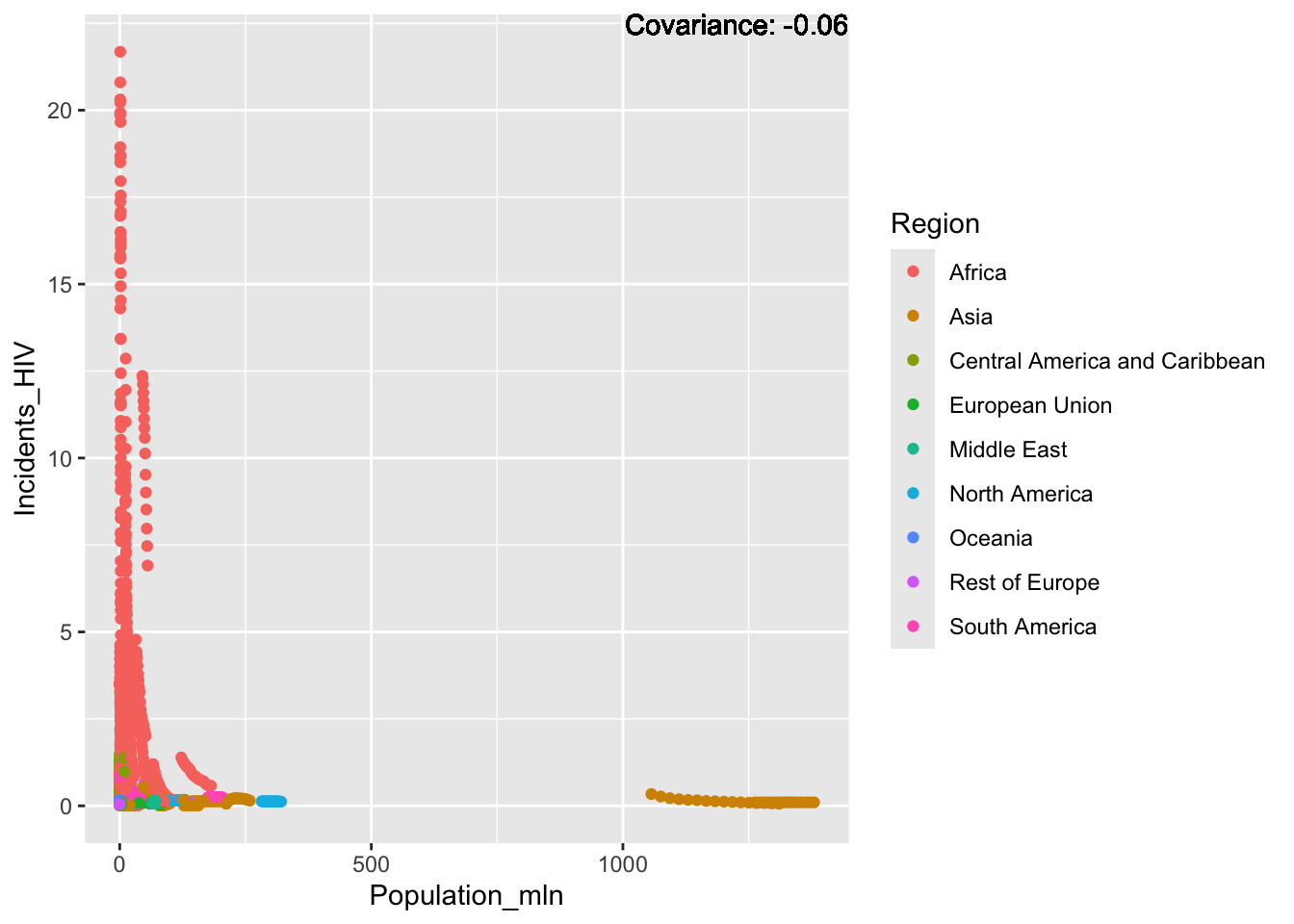

covariance_plot("Incidents_HIV", "Thinness_ten_nineteen_years", df, sdf)

Warning in geom_text(aes(label = paste("Covariance:", round(cov(std_data_frame[[y_val]], : All aesthetics have length 1, but the data has 2864 rows.
ℹ Please consider using `annotate()` or provide this layer with data containing
  a single row.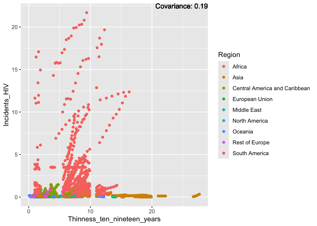

covariance_plot("Incidents_HIV", "Thinness_five_nine_years", df, sdf)

Warning in geom_text(aes(label = paste("Covariance:", round(cov(std_data_frame[[y_val]], : All aesthetics have length 1, but the data has 2864 rows.
ℹ Please consider using `annotate()` or provide this layer with data containing
  a single row.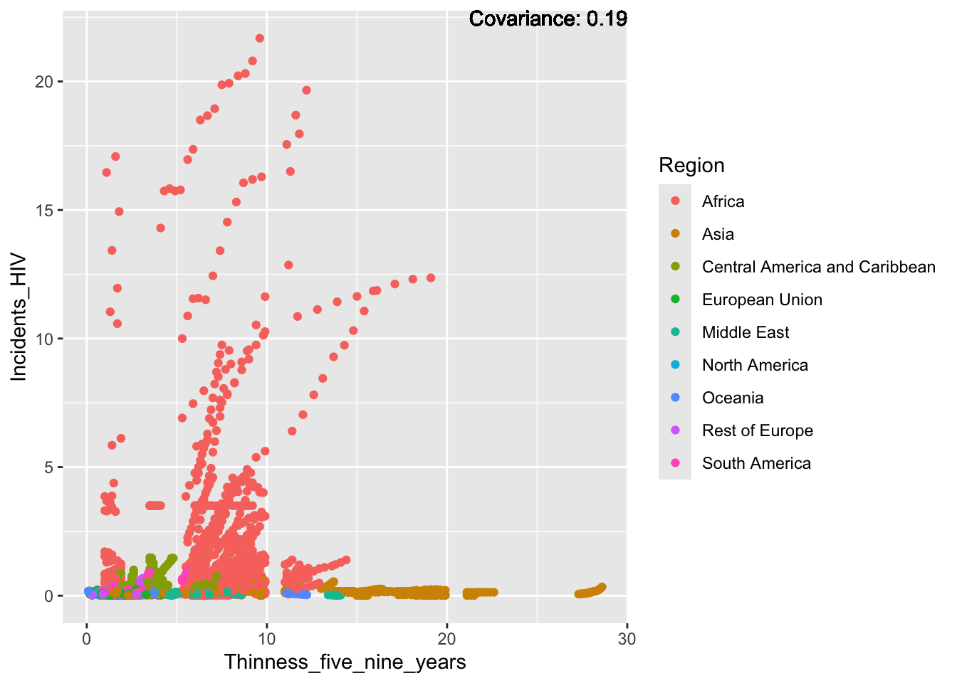

covariance_plot("Incidents_HIV", "Schooling", df, sdf)

Warning in geom_text(aes(label = paste("Covariance:", round(cov(std_data_frame[[y_val]], : All aesthetics have length 1, but the data has 2864 rows.
ℹ Please consider using `annotate()` or provide this layer with data containing
  a single row.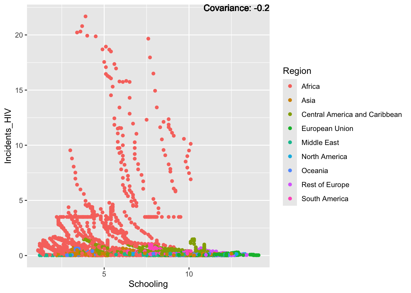

HIV Inferences:

Positive: Adult mortality

Negative: life expectancy

Conclusion: We may want to separate out Africa for this one, as it seems to be skewing the data.

Population:

covariance_plot("Population_mln", "GDP_per_capita", df, sdf)

Warning in geom_text(aes(label = paste("Covariance:", round(cov(std_data_frame[[y_val]], : All aesthetics have length 1, but the data has 2864 rows.
ℹ Please consider using `annotate()` or provide this layer with data containing
  a single row.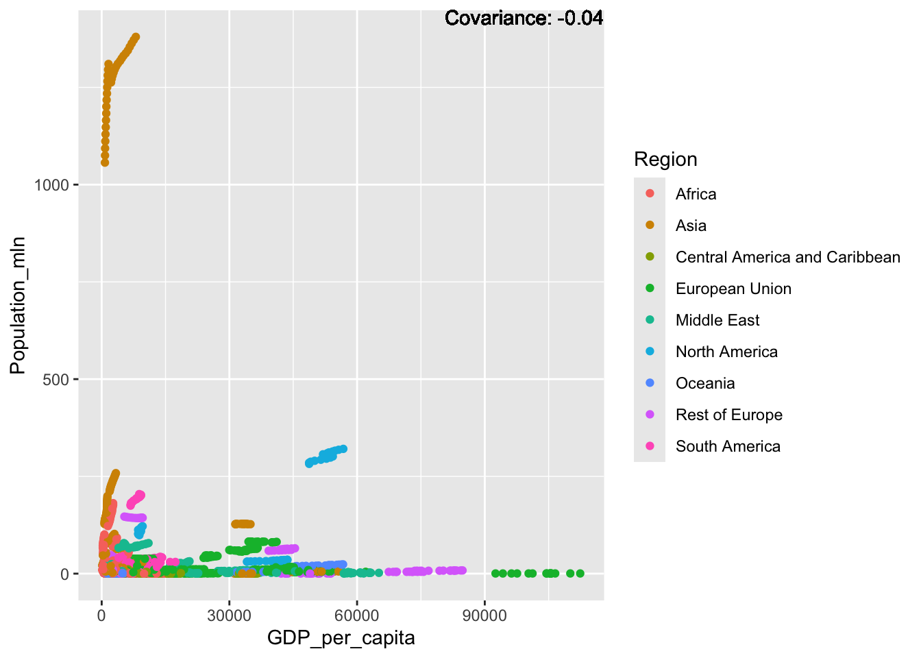

covariance_plot("Population_mln", "Infant_deaths", df, sdf)

Warning in geom_text(aes(label = paste("Covariance:", round(cov(std_data_frame[[y_val]], : All aesthetics have length 1, but the data has 2864 rows.
ℹ Please consider using `annotate()` or provide this layer with data containing
  a single row.

covariance_plot("Population_mln", "Under_five_deaths", df, sdf)

Warning in geom_text(aes(label = paste("Covariance:", round(cov(std_data_frame[[y_val]], : All aesthetics have length 1, but the data has 2864 rows.
ℹ Please consider using `annotate()` or provide this layer with data containing
  a single row.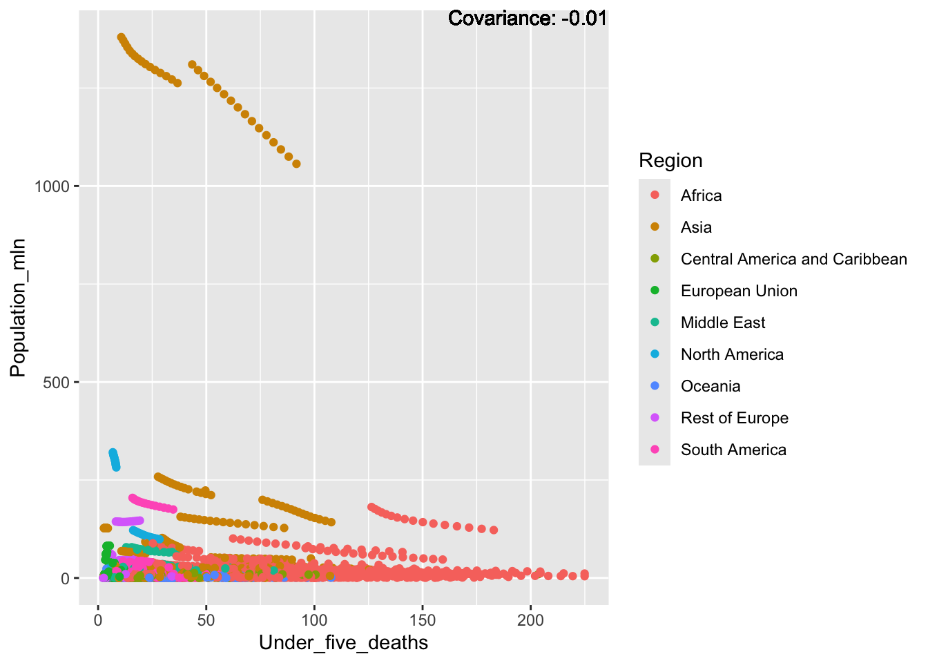

covariance_plot("Population_mln", "Life_expectancy", df, sdf)

Warning in geom_text(aes(label = paste("Covariance:", round(cov(std_data_frame[[y_val]], : All aesthetics have length 1, but the data has 2864 rows.
ℹ Please consider using `annotate()` or provide this layer with data containing
  a single row.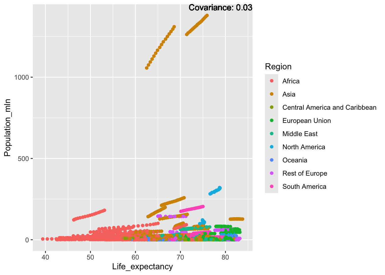

covariance_plot("Population_mln", "Adult_mortality", df, sdf)

Warning in geom_text(aes(label = paste("Covariance:", round(cov(std_data_frame[[y_val]], : All aesthetics have length 1, but the data has 2864 rows.
ℹ Please consider using `annotate()` or provide this layer with data containing
  a single row.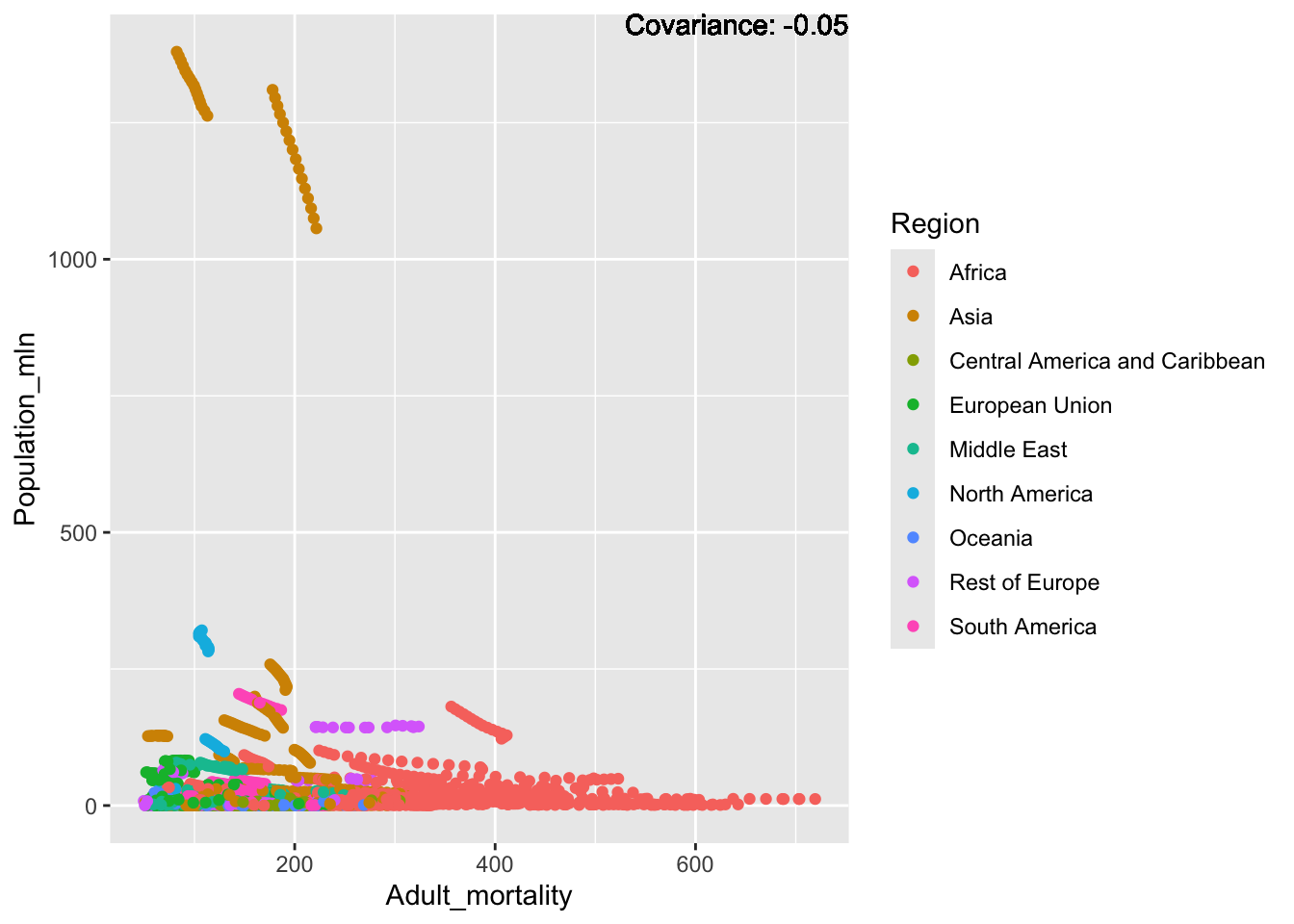

covariance_plot("Population_mln", "Hepatitis_B", df, sdf)

Warning in geom_text(aes(label = paste("Covariance:", round(cov(std_data_frame[[y_val]], : All aesthetics have length 1, but the data has 2864 rows.
ℹ Please consider using `annotate()` or provide this layer with data containing
  a single row.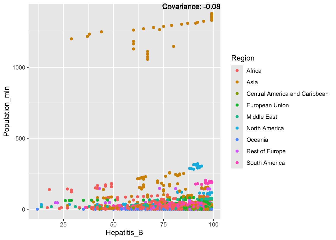

covariance_plot("Population_mln", "Measles", df, sdf)

Warning in geom_text(aes(label = paste("Covariance:", round(cov(std_data_frame[[y_val]], : All aesthetics have length 1, but the data has 2864 rows.
ℹ Please consider using `annotate()` or provide this layer with data containing
  a single row.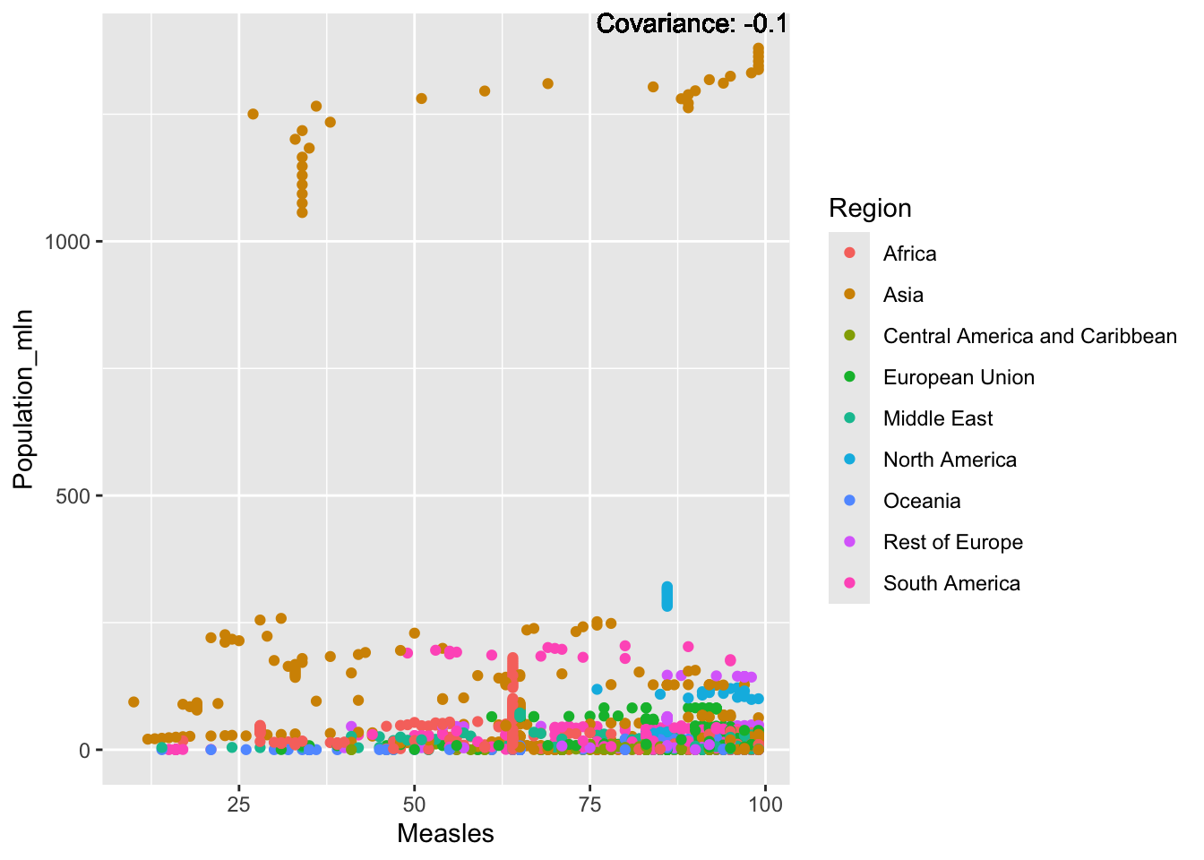

covariance_plot("Population_mln", "BMI", df, sdf)

Warning in geom_text(aes(label = paste("Covariance:", round(cov(std_data_frame[[y_val]], : All aesthetics have length 1, but the data has 2864 rows.
ℹ Please consider using `annotate()` or provide this layer with data containing
  a single row.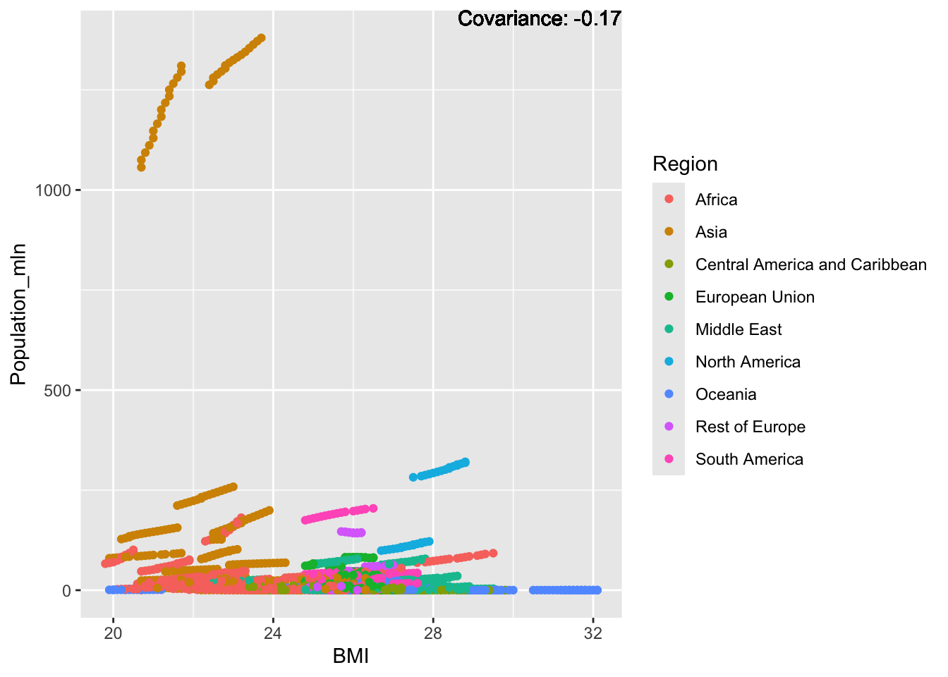

covariance_plot("Population_mln", "Polio", df, sdf)

Warning in geom_text(aes(label = paste("Covariance:", round(cov(std_data_frame[[y_val]], : All aesthetics have length 1, but the data has 2864 rows.
ℹ Please consider using `annotate()` or provide this layer with data containing
  a single row.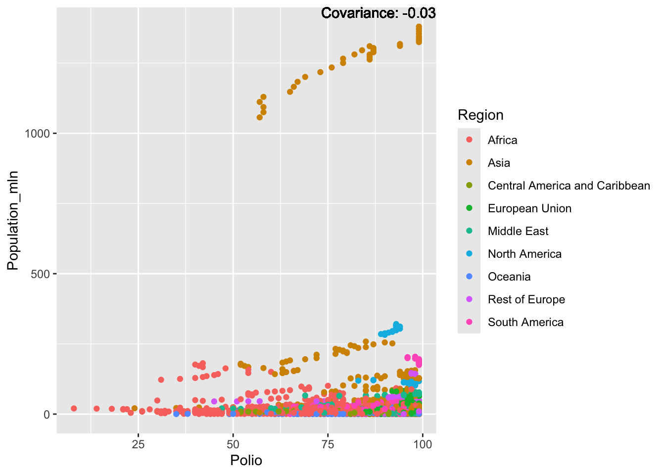

covariance_plot("Population_mln", "Diphtheria", df, sdf)

Warning in geom_text(aes(label = paste("Covariance:", round(cov(std_data_frame[[y_val]], : All aesthetics have length 1, but the data has 2864 rows.
ℹ Please consider using `annotate()` or provide this layer with data containing
  a single row.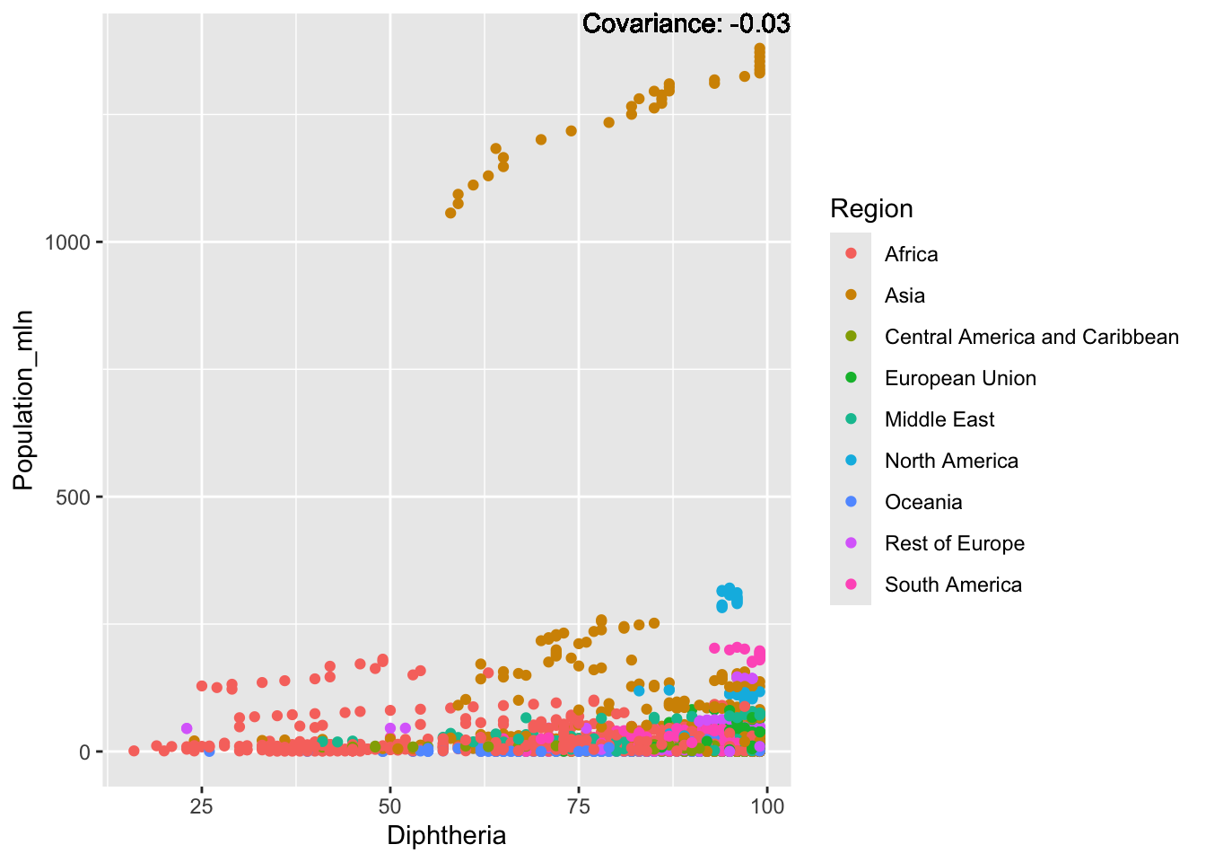

covariance_plot("Population_mln", "Alcohol_consumption", df, sdf)

Warning in geom_text(aes(label = paste("Covariance:", round(cov(std_data_frame[[y_val]], : All aesthetics have length 1, but the data has 2864 rows.
ℹ Please consider using `annotate()` or provide this layer with data containing
  a single row.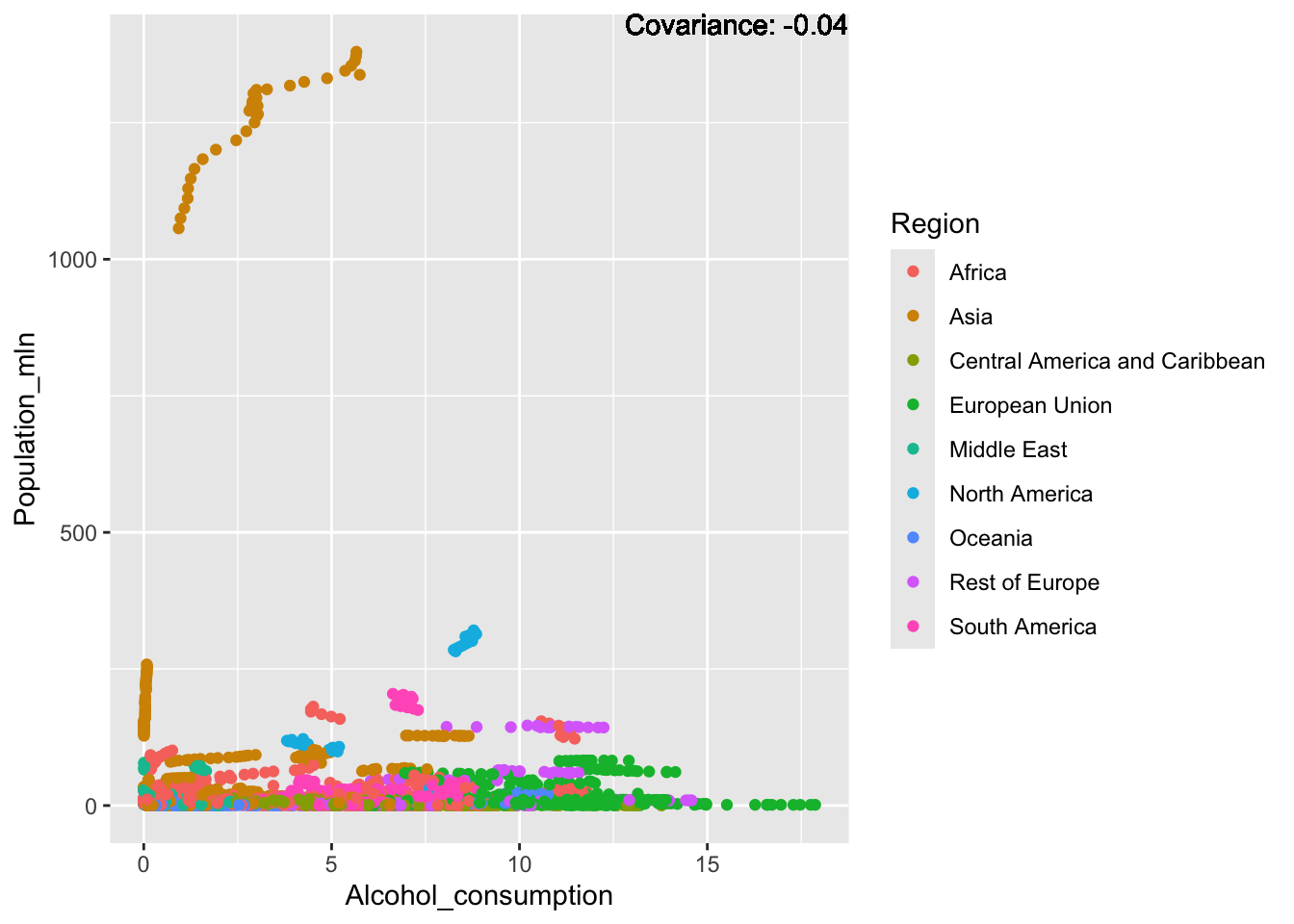

covariance_plot("Population_mln", "Incidents_HIV", df, sdf)

Warning in geom_text(aes(label = paste("Covariance:", round(cov(std_data_frame[[y_val]], : All aesthetics have length 1, but the data has 2864 rows.
ℹ Please consider using `annotate()` or provide this layer with data containing
  a single row.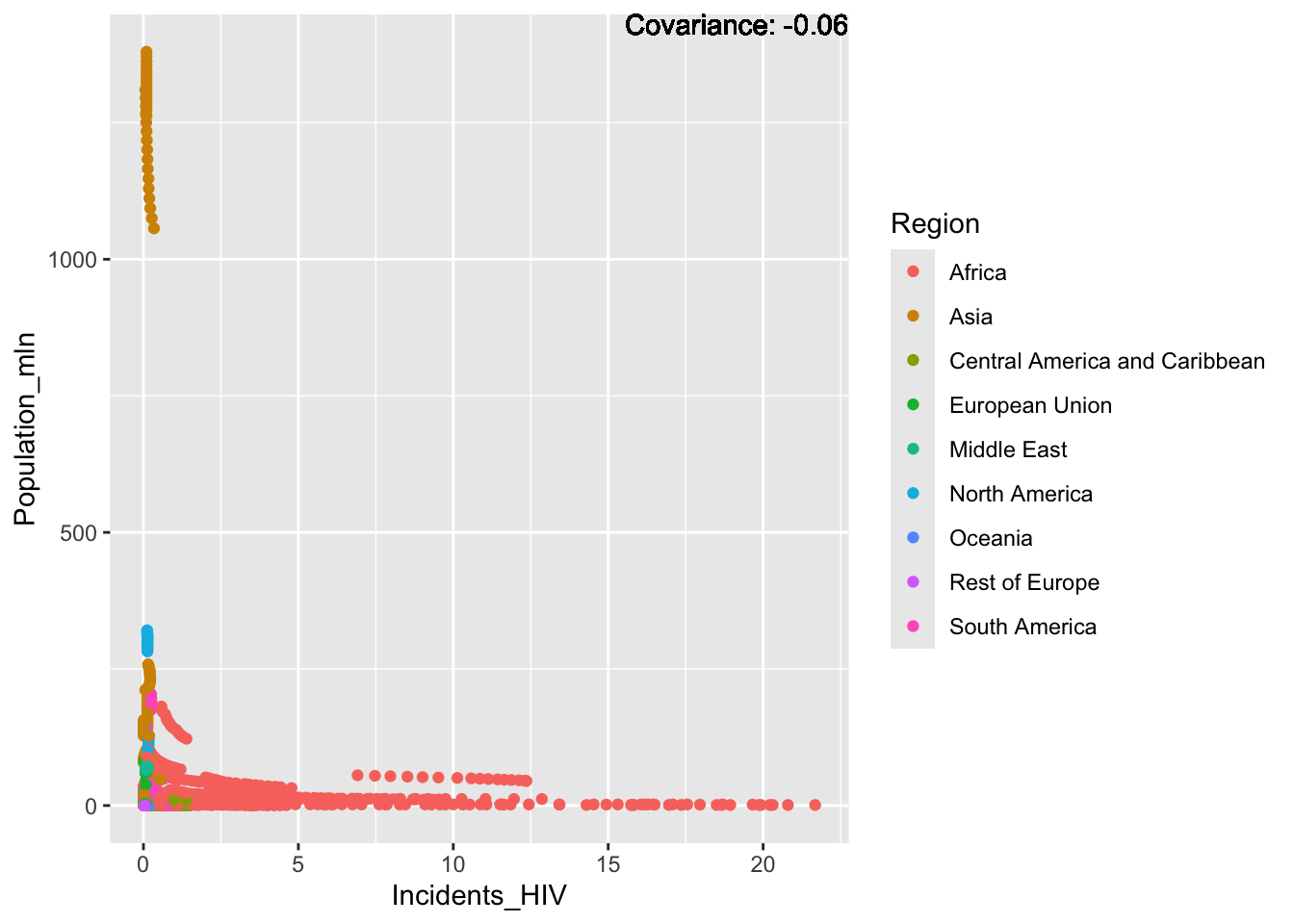

covariance_plot("Population_mln", "Thinness_ten_nineteen_years", df, sdf)

Warning in geom_text(aes(label = paste("Covariance:", round(cov(std_data_frame[[y_val]], : All aesthetics have length 1, but the data has 2864 rows.
ℹ Please consider using `annotate()` or provide this layer with data containing
  a single row.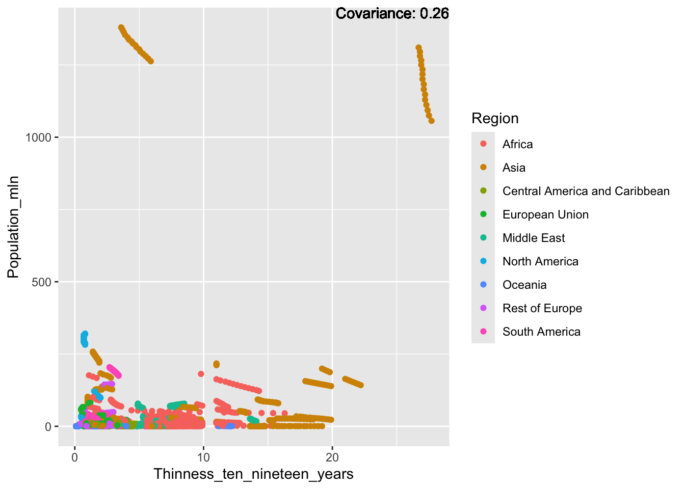

covariance_plot("Population_mln", "Thinness_five_nine_years", df, sdf)

Warning in geom_text(aes(label = paste("Covariance:", round(cov(std_data_frame[[y_val]], : All aesthetics have length 1, but the data has 2864 rows.
ℹ Please consider using `annotate()` or provide this layer with data containing
  a single row.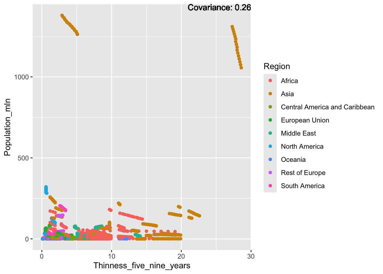

covariance_plot("Population_mln", "Schooling", df, sdf)

Warning in geom_text(aes(label = paste("Covariance:", round(cov(std_data_frame[[y_val]], : All aesthetics have length 1, but the data has 2864 rows.
ℹ Please consider using `annotate()` or provide this layer with data containing
  a single row.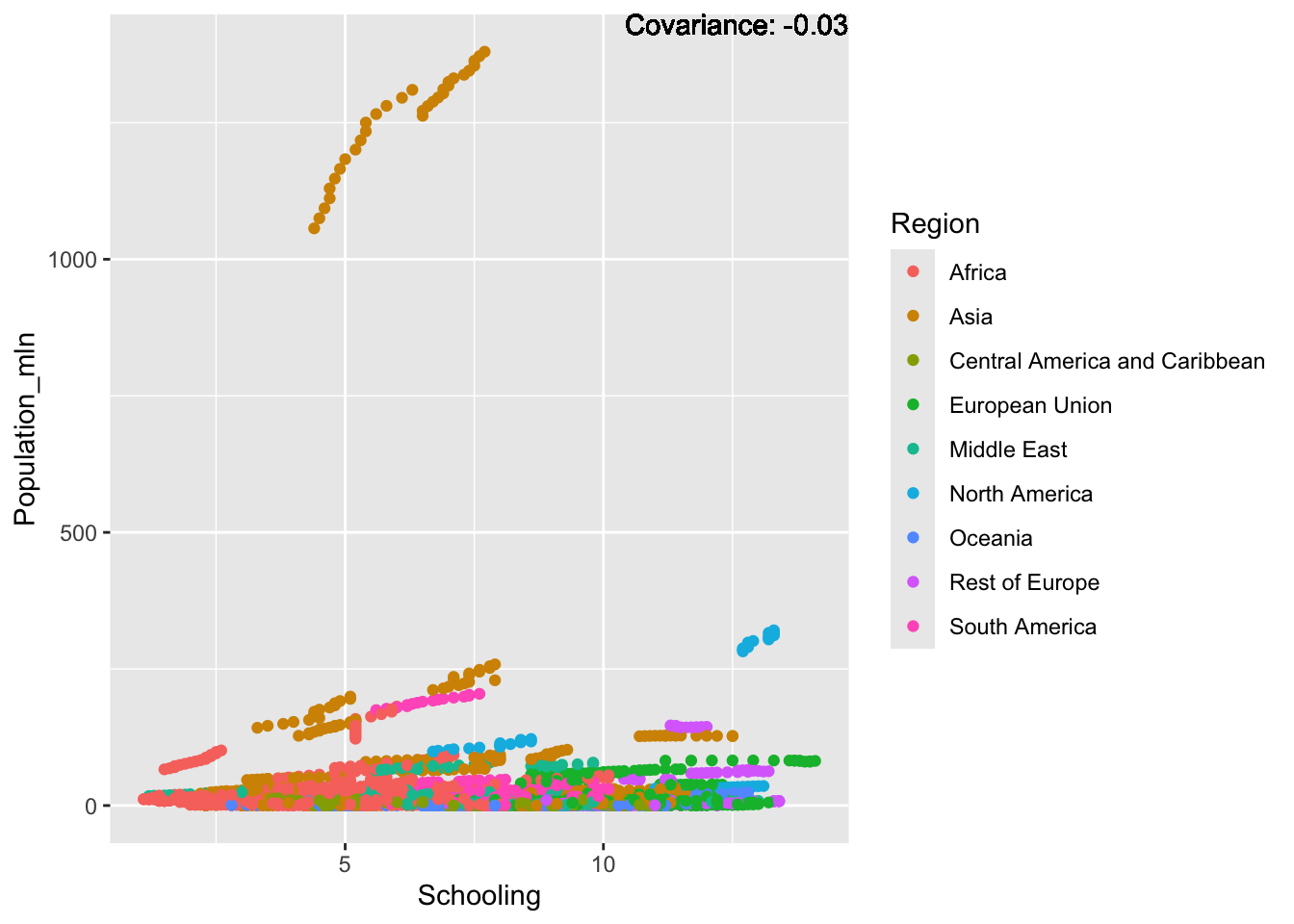

Population Inferences:

Conclusion: We may want to do this again without China and India, as they seems to be skewing the data

Thinness:

covariance_plot("Thinness_ten_nineteen_years", "GDP_per_capita", df, sdf)

Warning in geom_text(aes(label = paste("Covariance:", round(cov(std_data_frame[[y_val]], : All aesthetics have length 1, but the data has 2864 rows.
ℹ Please consider using `annotate()` or provide this layer with data containing
  a single row.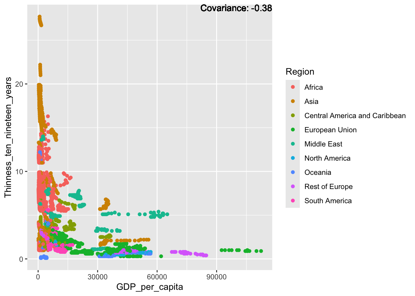

covariance_plot("Thinness_ten_nineteen_years", "Infant_deaths", df, sdf)

Warning in geom_text(aes(label = paste("Covariance:", round(cov(std_data_frame[[y_val]], : All aesthetics have length 1, but the data has 2864 rows.
ℹ Please consider using `annotate()` or provide this layer with data containing
  a single row.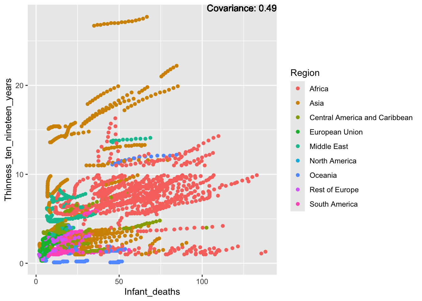

covariance_plot("Thinness_ten_nineteen_years", "Under_five_deaths", df, sdf)

Warning in geom_text(aes(label = paste("Covariance:", round(cov(std_data_frame[[y_val]], : All aesthetics have length 1, but the data has 2864 rows.
ℹ Please consider using `annotate()` or provide this layer with data containing
  a single row.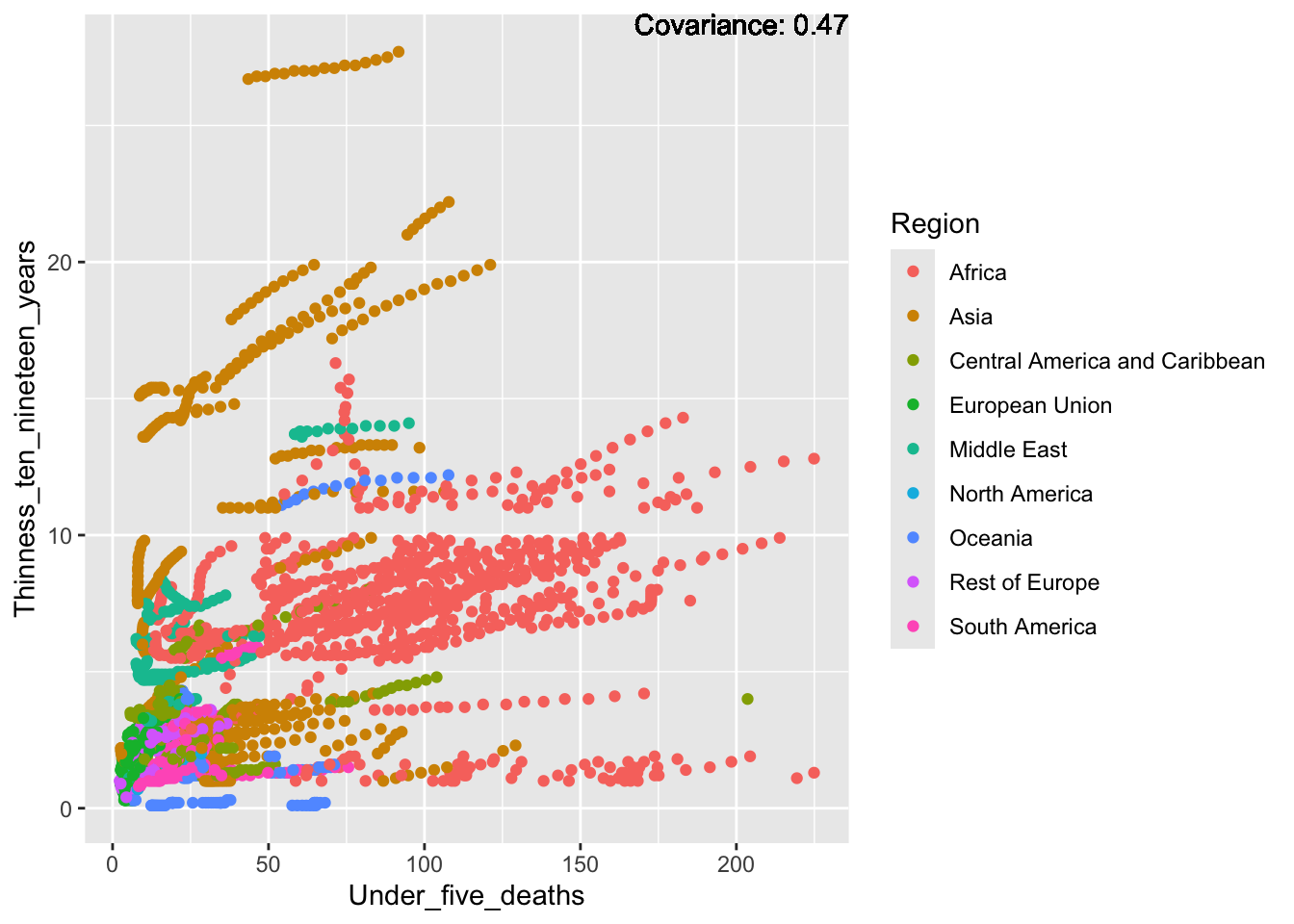

covariance_plot("Thinness_ten_nineteen_years", "Life_expectancy", df, sdf)

Warning in geom_text(aes(label = paste("Covariance:", round(cov(std_data_frame[[y_val]], : All aesthetics have length 1, but the data has 2864 rows.
ℹ Please consider using `annotate()` or provide this layer with data containing
  a single row.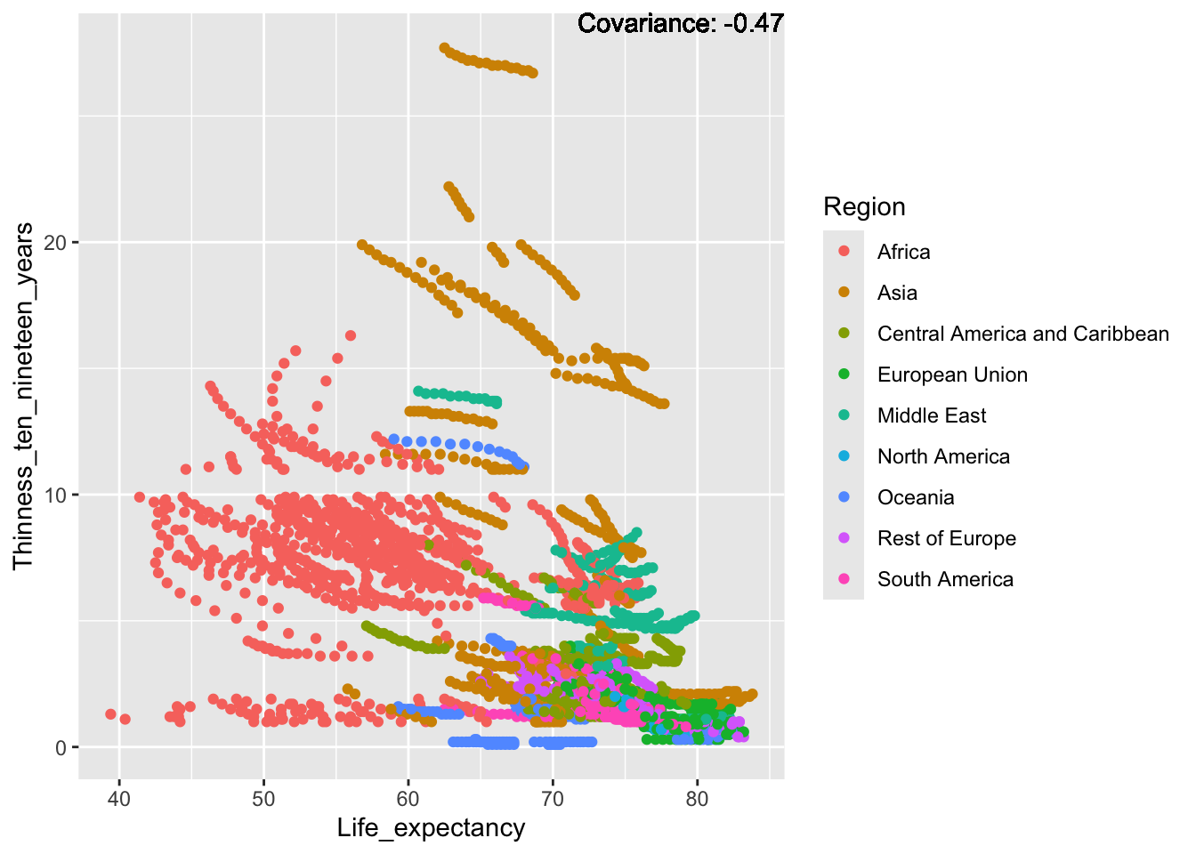

covariance_plot("Thinness_ten_nineteen_years", "Adult_mortality", df, sdf)

Warning in geom_text(aes(label = paste("Covariance:", round(cov(std_data_frame[[y_val]], : All aesthetics have length 1, but the data has 2864 rows.
ℹ Please consider using `annotate()` or provide this layer with data containing
  a single row.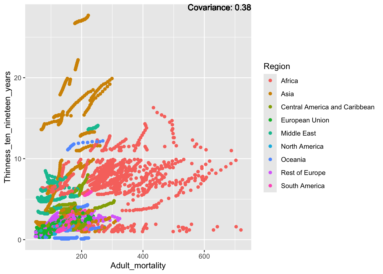

covariance_plot("Thinness_ten_nineteen_years", "Hepatitis_B", df, sdf)

Warning in geom_text(aes(label = paste("Covariance:", round(cov(std_data_frame[[y_val]], : All aesthetics have length 1, but the data has 2864 rows.
ℹ Please consider using `annotate()` or provide this layer with data containing
  a single row.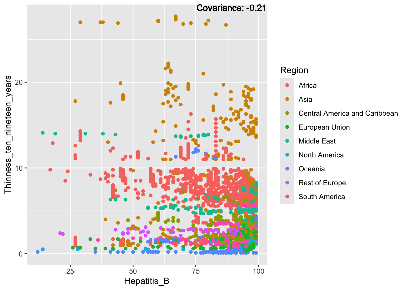

covariance_plot("Thinness_ten_nineteen_years", "Measles", df, sdf)

Warning in geom_text(aes(label = paste("Covariance:", round(cov(std_data_frame[[y_val]], : All aesthetics have length 1, but the data has 2864 rows.
ℹ Please consider using `annotate()` or provide this layer with data containing
  a single row.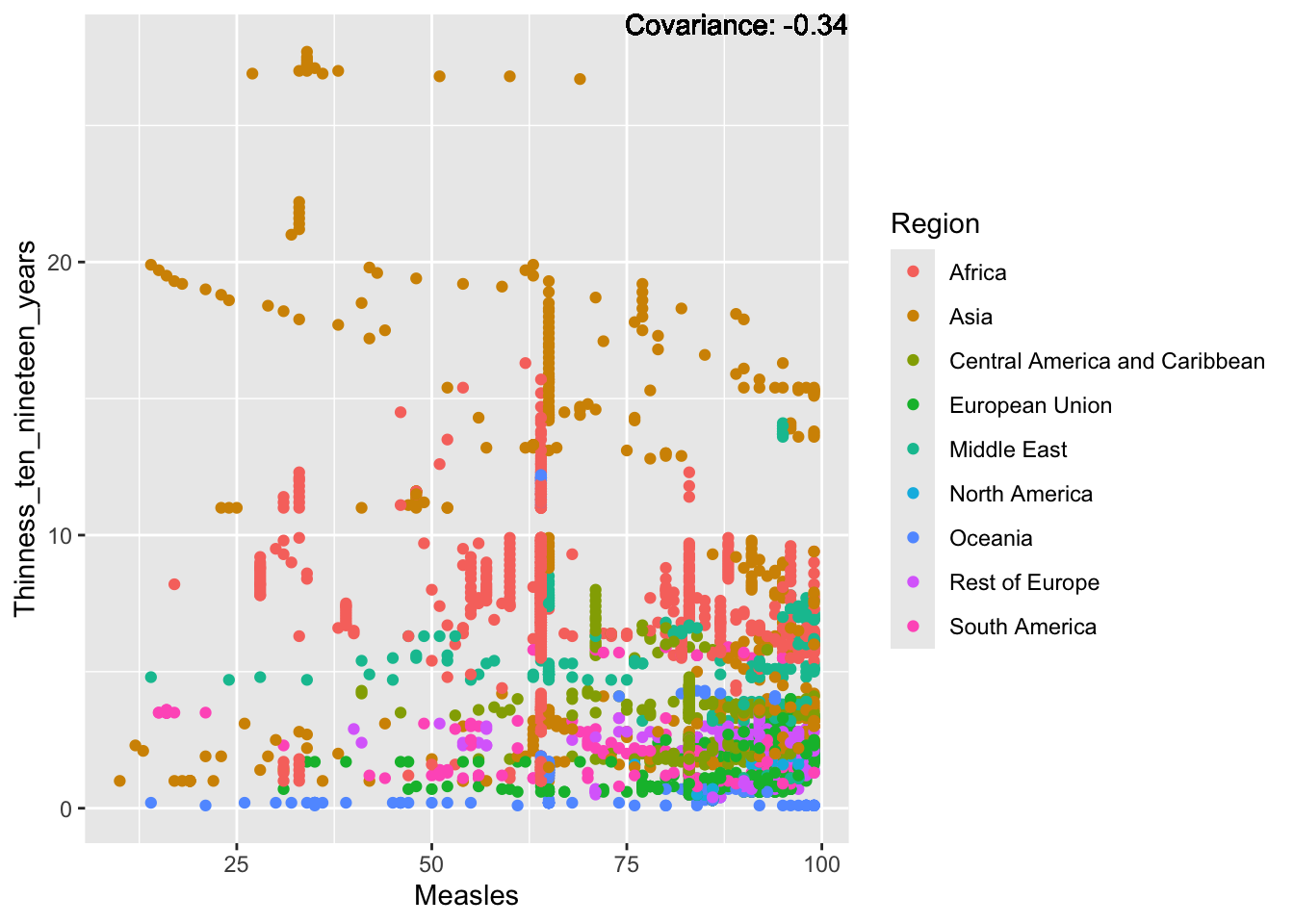

covariance_plot("Thinness_ten_nineteen_years", "BMI", df, sdf)

Warning in geom_text(aes(label = paste("Covariance:", round(cov(std_data_frame[[y_val]], : All aesthetics have length 1, but the data has 2864 rows.
ℹ Please consider using `annotate()` or provide this layer with data containing
  a single row.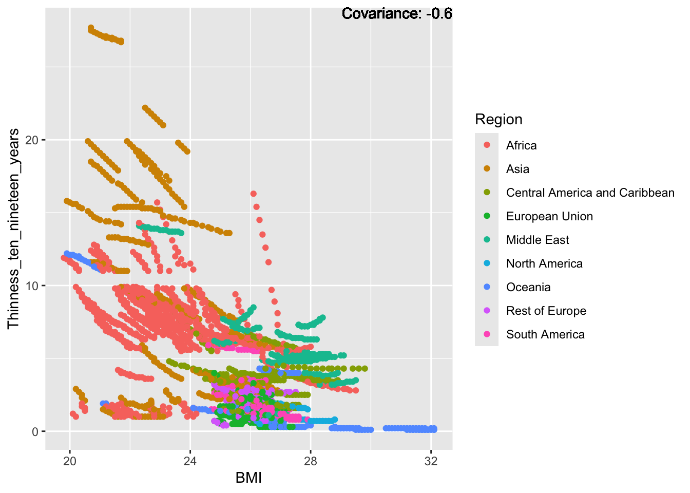

covariance_plot("Thinness_ten_nineteen_years", "Polio", df, sdf)

Warning in geom_text(aes(label = paste("Covariance:", round(cov(std_data_frame[[y_val]], : All aesthetics have length 1, but the data has 2864 rows.
ℹ Please consider using `annotate()` or provide this layer with data containing
  a single row.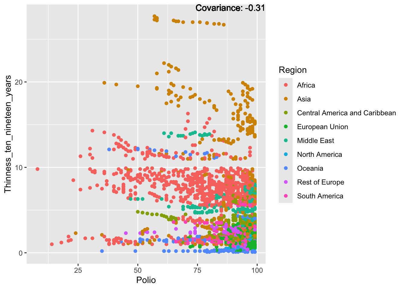

covariance_plot("Thinness_ten_nineteen_years", "Diphtheria", df, sdf)

Warning in geom_text(aes(label = paste("Covariance:", round(cov(std_data_frame[[y_val]], : All aesthetics have length 1, but the data has 2864 rows.
ℹ Please consider using `annotate()` or provide this layer with data containing
  a single row.

covariance_plot("Thinness_ten_nineteen_years", "Alcohol_consumption", df, sdf)

Warning in geom_text(aes(label = paste("Covariance:", round(cov(std_data_frame[[y_val]], : All aesthetics have length 1, but the data has 2864 rows.
ℹ Please consider using `annotate()` or provide this layer with data containing
  a single row.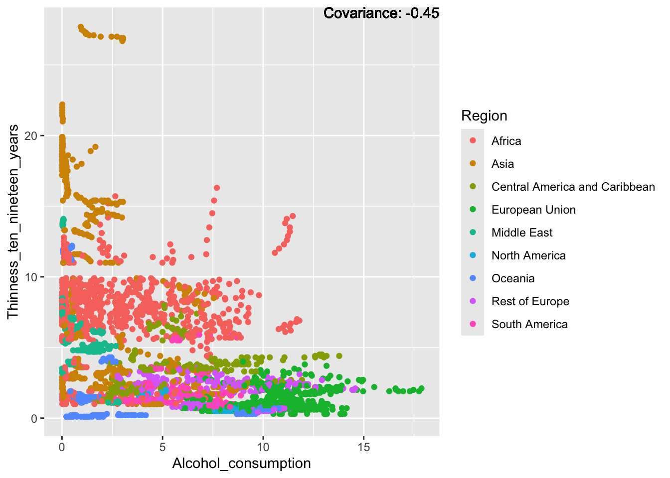

covariance_plot("Thinness_ten_nineteen_years", "Incidents_HIV", df, sdf)

Warning in geom_text(aes(label = paste("Covariance:", round(cov(std_data_frame[[y_val]], : All aesthetics have length 1, but the data has 2864 rows.
ℹ Please consider using `annotate()` or provide this layer with data containing
  a single row.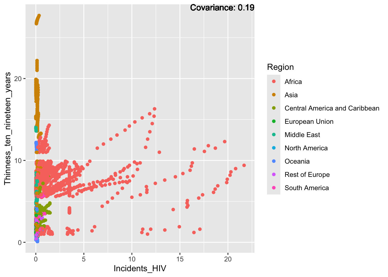

covariance_plot("Thinness_ten_nineteen_years", "Population_mln", df, sdf)

Warning in geom_text(aes(label = paste("Covariance:", round(cov(std_data_frame[[y_val]], : All aesthetics have length 1, but the data has 2864 rows.
ℹ Please consider using `annotate()` or provide this layer with data containing
  a single row.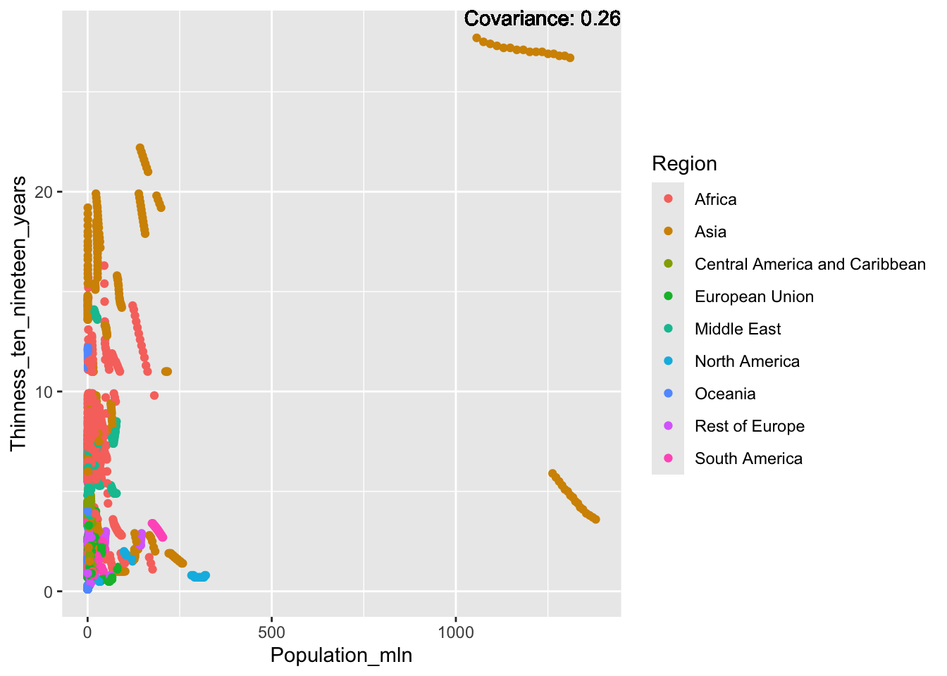

covariance_plot("Thinness_ten_nineteen_years", "Thinness_five_nine_years", df, sdf)

Warning in geom_text(aes(label = paste("Covariance:", round(cov(std_data_frame[[y_val]], : All aesthetics have length 1, but the data has 2864 rows.
ℹ Please consider using `annotate()` or provide this layer with data containing
  a single row.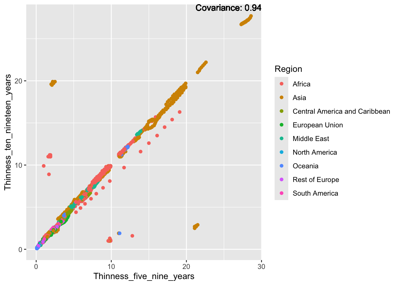

covariance_plot("Thinness_ten_nineteen_years", "Schooling", df, sdf)

Warning in geom_text(aes(label = paste("Covariance:", round(cov(std_data_frame[[y_val]], : All aesthetics have length 1, but the data has 2864 rows.
ℹ Please consider using `annotate()` or provide this layer with data containing
  a single row.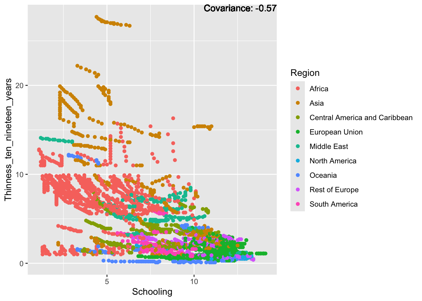

Thinness:

Strong positive: Thinness

Positive: Infant deaths, under five deaths, adult mortality

Negative: Life expectancy, alcohol consumption, BMI, schooling

No surprise that the two thinness are basically one to one.

Schooling:

covariance_plot("Schooling", "GDP_per_capita", df, sdf)

Warning in geom_text(aes(label = paste("Covariance:", round(cov(std_data_frame[[y_val]], : All aesthetics have length 1, but the data has 2864 rows.
ℹ Please consider using `annotate()` or provide this layer with data containing
  a single row.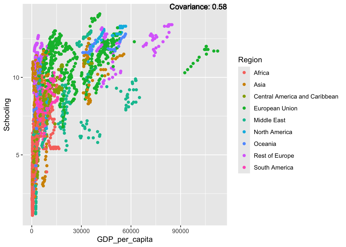

covariance_plot("Schooling", "Infant_deaths", df, sdf)

Warning in geom_text(aes(label = paste("Covariance:", round(cov(std_data_frame[[y_val]], : All aesthetics have length 1, but the data has 2864 rows.
ℹ Please consider using `annotate()` or provide this layer with data containing
  a single row.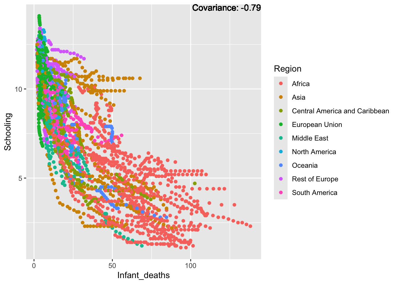

covariance_plot("Schooling", "Under_five_deaths", df, sdf)

Warning in geom_text(aes(label = paste("Covariance:", round(cov(std_data_frame[[y_val]], : All aesthetics have length 1, but the data has 2864 rows.
ℹ Please consider using `annotate()` or provide this layer with data containing
  a single row.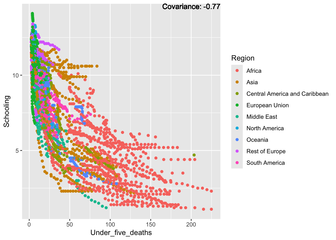

covariance_plot("Schooling", "Life_expectancy", df, sdf)

Warning in geom_text(aes(label = paste("Covariance:", round(cov(std_data_frame[[y_val]], : All aesthetics have length 1, but the data has 2864 rows.
ℹ Please consider using `annotate()` or provide this layer with data containing
  a single row.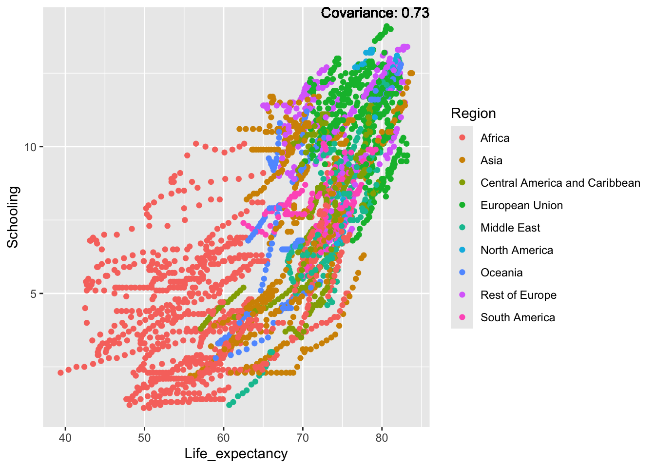

covariance_plot("Schooling", "Adult_mortality", df, sdf)

Warning in geom_text(aes(label = paste("Covariance:", round(cov(std_data_frame[[y_val]], : All aesthetics have length 1, but the data has 2864 rows.
ℹ Please consider using `annotate()` or provide this layer with data containing
  a single row.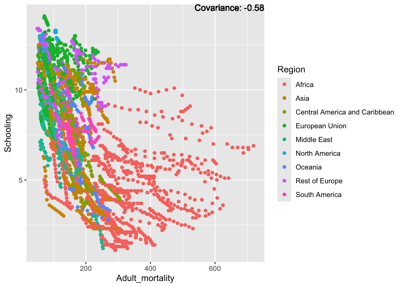

covariance_plot("Schooling", "Hepatitis_B", df, sdf)

Warning in geom_text(aes(label = paste("Covariance:", round(cov(std_data_frame[[y_val]], : All aesthetics have length 1, but the data has 2864 rows.
ℹ Please consider using `annotate()` or provide this layer with data containing
  a single row.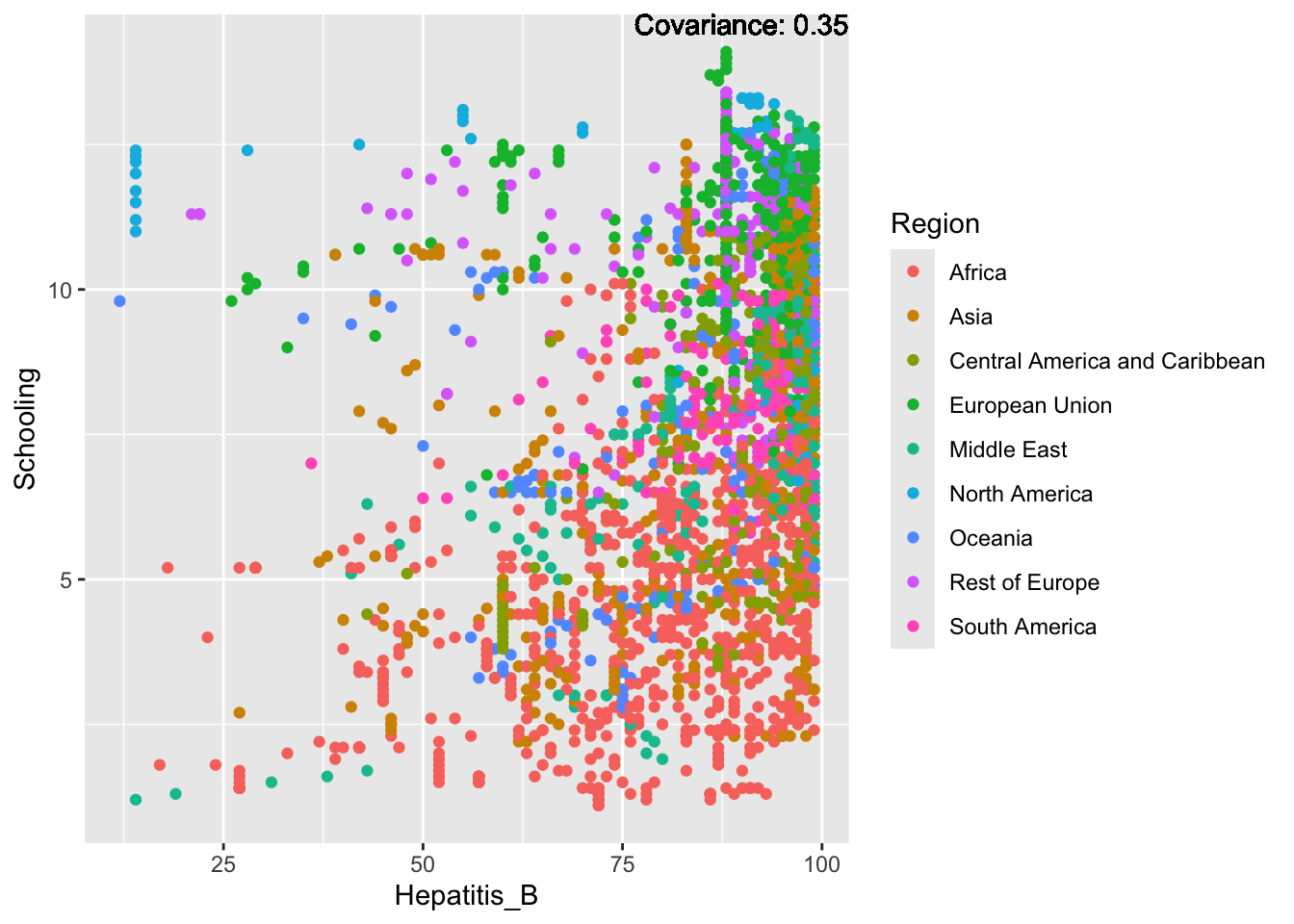

covariance_plot("Schooling", "Measles", df, sdf)

Warning in geom_text(aes(label = paste("Covariance:", round(cov(std_data_frame[[y_val]], : All aesthetics have length 1, but the data has 2864 rows.
ℹ Please consider using `annotate()` or provide this layer with data containing
  a single row.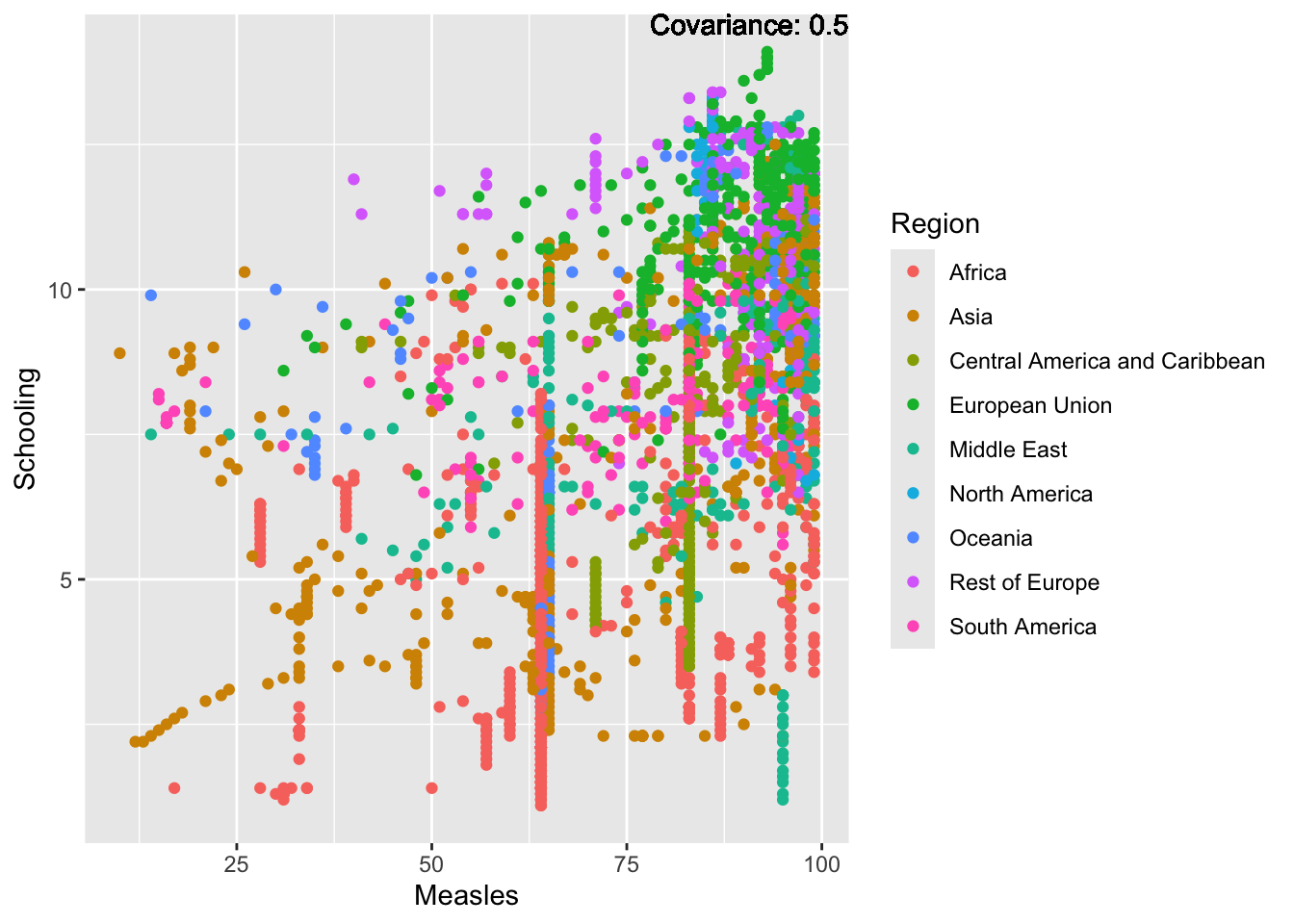

covariance_plot("Schooling", "BMI", df, sdf)

Warning in geom_text(aes(label = paste("Covariance:", round(cov(std_data_frame[[y_val]], : All aesthetics have length 1, but the data has 2864 rows.
ℹ Please consider using `annotate()` or provide this layer with data containing
  a single row.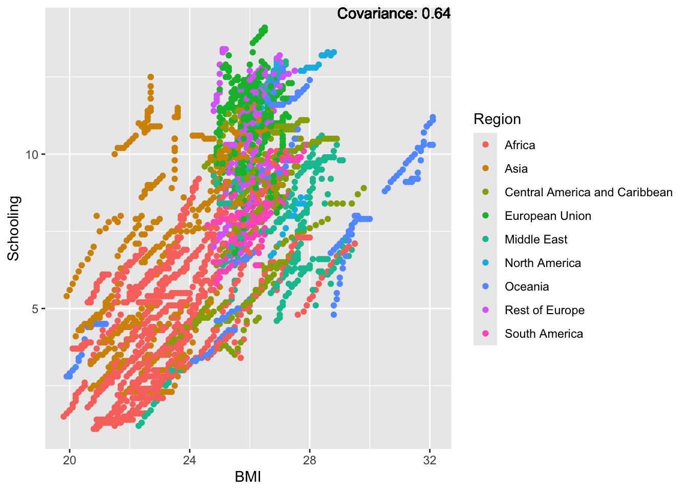

covariance_plot("Schooling", "Polio", df, sdf)

Warning in geom_text(aes(label = paste("Covariance:", round(cov(std_data_frame[[y_val]], : All aesthetics have length 1, but the data has 2864 rows.
ℹ Please consider using `annotate()` or provide this layer with data containing
  a single row.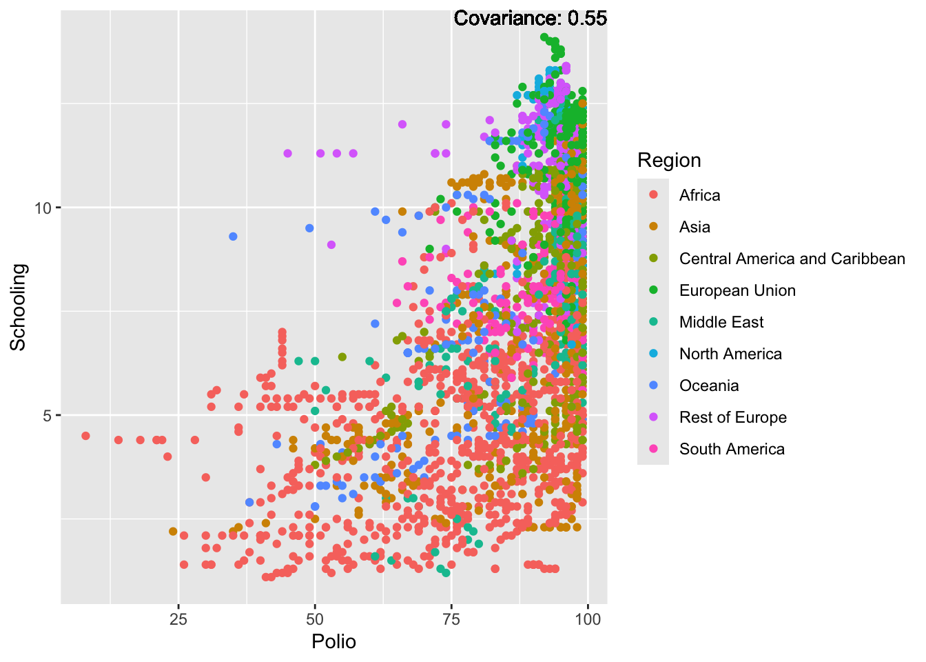

covariance_plot("Schooling", "Diphtheria", df, sdf)

Warning in geom_text(aes(label = paste("Covariance:", round(cov(std_data_frame[[y_val]], : All aesthetics have length 1, but the data has 2864 rows.
ℹ Please consider using `annotate()` or provide this layer with data containing
  a single row.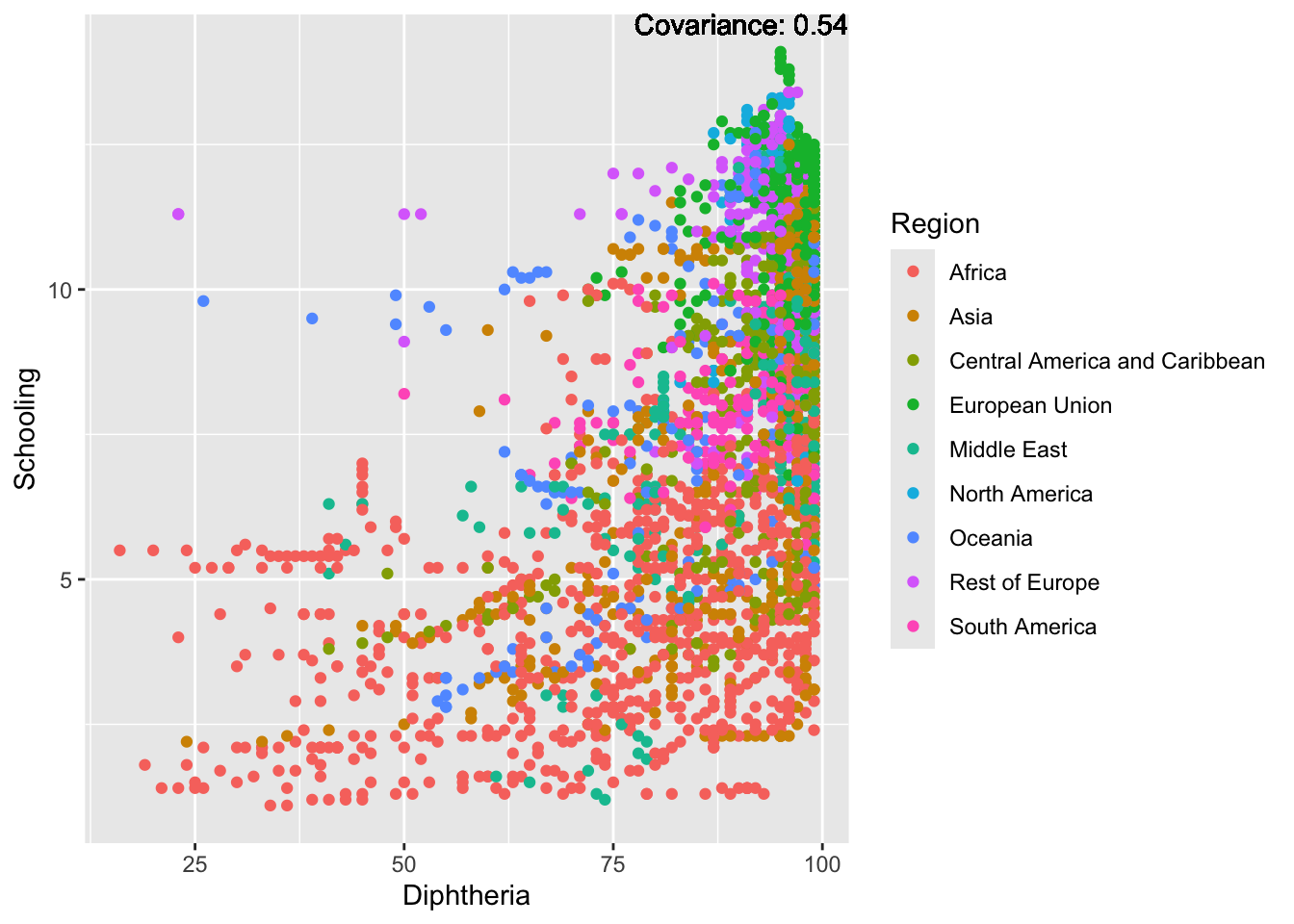

covariance_plot("Schooling", "Alcohol_consumption", df, sdf)

Warning in geom_text(aes(label = paste("Covariance:", round(cov(std_data_frame[[y_val]], : All aesthetics have length 1, but the data has 2864 rows.
ℹ Please consider using `annotate()` or provide this layer with data containing
  a single row.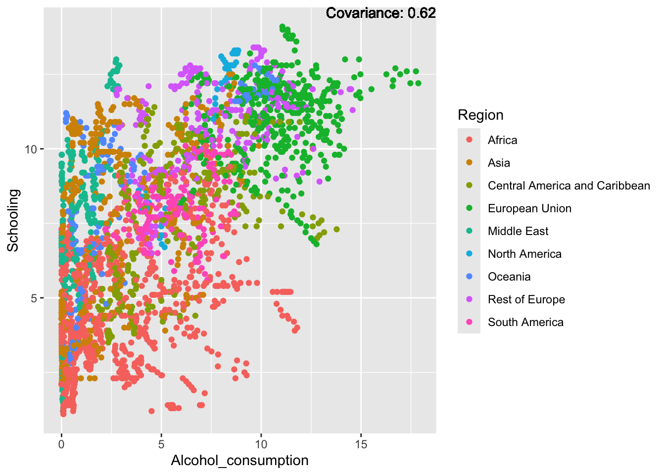

covariance_plot("Schooling", "Incidents_HIV", df, sdf)

Warning in geom_text(aes(label = paste("Covariance:", round(cov(std_data_frame[[y_val]], : All aesthetics have length 1, but the data has 2864 rows.
ℹ Please consider using `annotate()` or provide this layer with data containing
  a single row.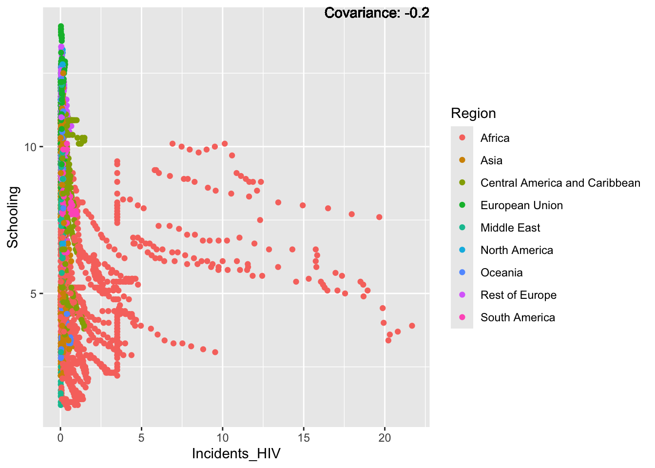

covariance_plot("Schooling", "Population_mln", df, sdf)

Warning in geom_text(aes(label = paste("Covariance:", round(cov(std_data_frame[[y_val]], : All aesthetics have length 1, but the data has 2864 rows.
ℹ Please consider using `annotate()` or provide this layer with data containing
  a single row.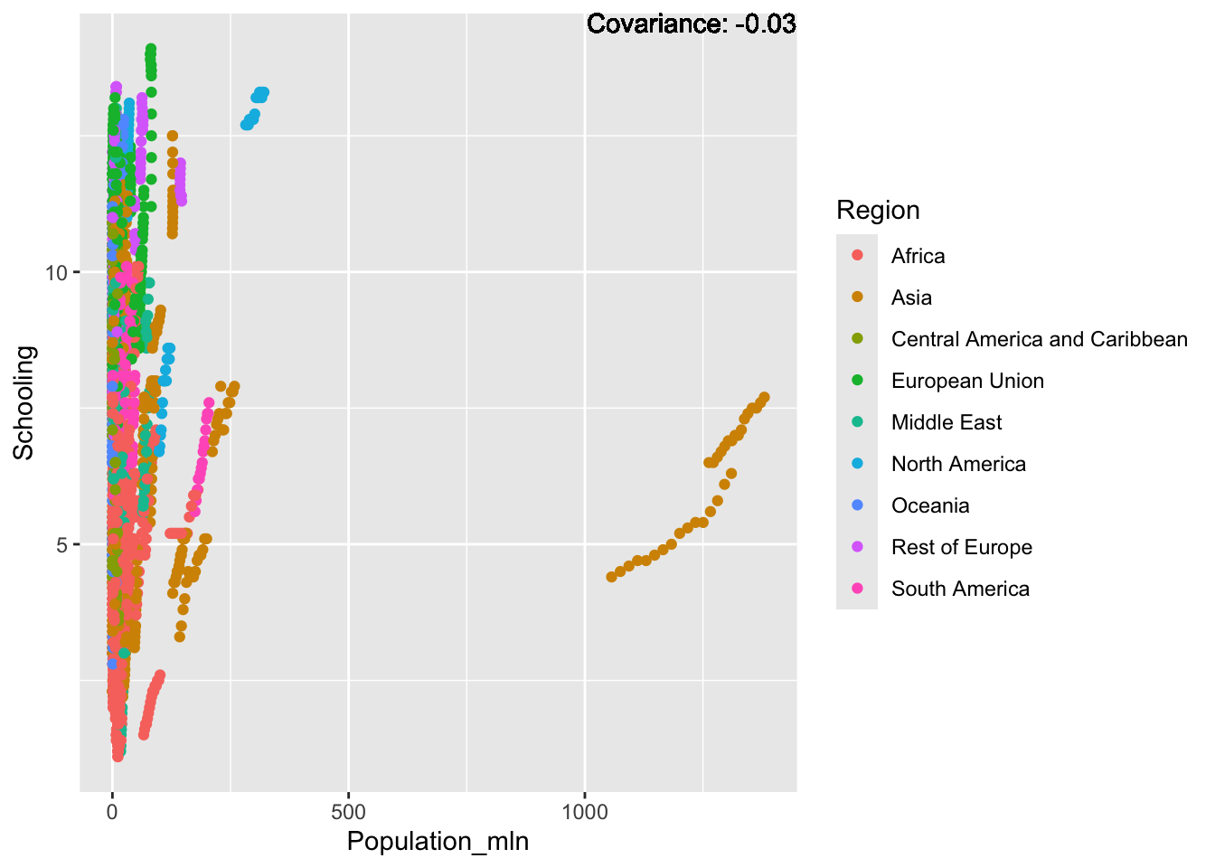

covariance_plot("Schooling", "Thinness_five_nine_years", df, sdf)

Warning in geom_text(aes(label = paste("Covariance:", round(cov(std_data_frame[[y_val]], : All aesthetics have length 1, but the data has 2864 rows.
ℹ Please consider using `annotate()` or provide this layer with data containing
  a single row.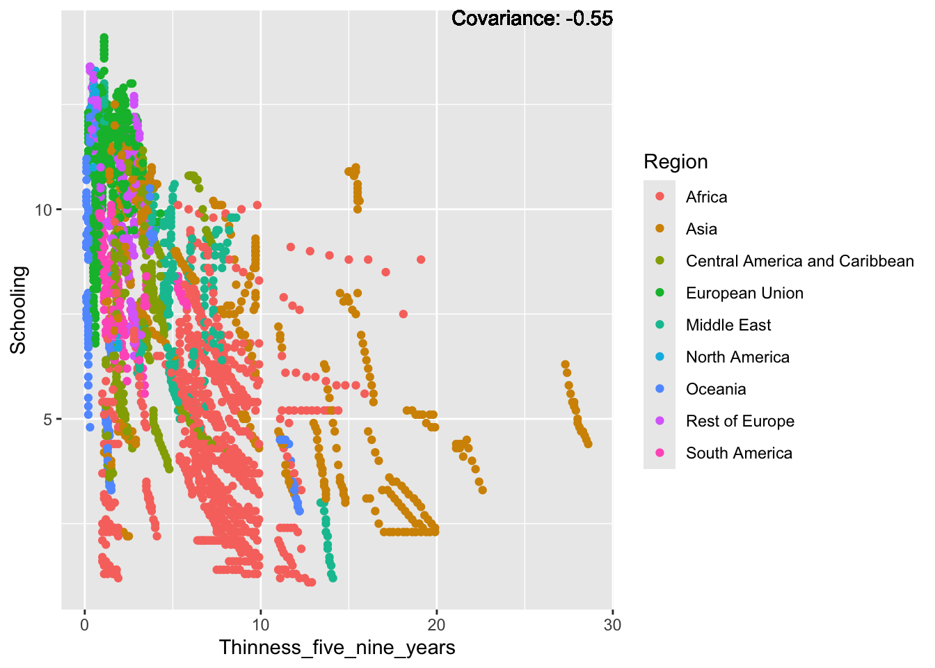

covariance_plot("Schooling", "Thinness_ten_nineteen_years", df, sdf)

Warning in geom_text(aes(label = paste("Covariance:", round(cov(std_data_frame[[y_val]], : All aesthetics have length 1, but the data has 2864 rows.
ℹ Please consider using `annotate()` or provide this layer with data containing
  a single row.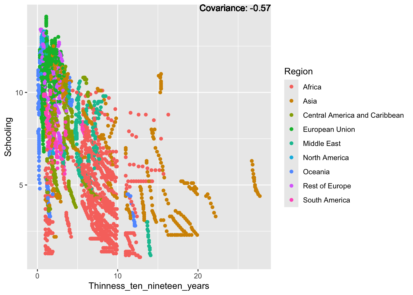

Inferences:

Positive: Life expectancy, alcohol consumption, measles, BMI, polio, diphtheria, GDP

Negative: Infant deaths, under five deaths, adult mortality, thinness

Models

5.1 Multiple Regression of Life Expectancy

For testing purposes, we must separate out a portion of the data now. We will be using a 80/20 split. 80% Training, 20% testing.

5.1.1 Splitting the Data

#seed to make this reproducible 
set.seed(333)

#split the data
training.samples <- sdf$Life_expectancy |> createDataPartition(p = 0.8, list = FALSE)

train.data <- sdf[training.samples, ]
test.data <- sdf[-training.samples, ]

5.1.2 Making the First Model

We are leaving out one of the two economy status variables as they are two halves of a binary variable.

We must also pick between Country and Region, as having both in the model seems to create singularities. For readability sake we will be keeping Region

#make the model
LE_MR <- lm(Life_expectancy ~ .  -Economy_status_Developing -Country , data = train.data)

#print summary of the model
summary(LE_MR)


Call:
lm(formula = Life_expectancy ~ . - Economy_status_Developing - 
    Country, data = train.data)

Residuals:
     Min       1Q   Median       3Q      Max 
-0.45439 -0.08736 -0.00297  0.08382  0.60675 

Coefficients:
                                      Estimate Std. Error t value Pr(>|t|)    
(Intercept)                         -0.1066983  0.0139377  -7.655 2.84e-14 ***
RegionAsia                           0.0408052  0.0121871   3.348 0.000827 ***
RegionCentral America and Caribbean  0.2160099  0.0128928  16.754  < 2e-16 ***
RegionEuropean Union                -0.0760235  0.0190799  -3.984 6.98e-05 ***
RegionMiddle East                    0.0337327  0.0149020   2.264 0.023691 *  
RegionNorth America                  0.0806516  0.0254903   3.164 0.001577 ** 
RegionOceania                       -0.0846981  0.0154317  -5.489 4.51e-08 ***
RegionRest of Europe                 0.0305305  0.0151715   2.012 0.044300 *  
RegionSouth America                  0.1913290  0.0148165  12.913  < 2e-16 ***
Infant_deaths                       -0.1453887  0.0179910  -8.081 1.04e-15 ***
Under_five_deaths                   -0.2410563  0.0181045 -13.315  < 2e-16 ***
Adult_mortality                     -0.5682994  0.0078518 -72.379  < 2e-16 ***
Alcohol_consumption                 -0.0015641  0.0049114  -0.318 0.750163    
Hepatitis_B                         -0.0132183  0.0045331  -2.916 0.003581 ** 
Measles                              0.0025920  0.0034613   0.749 0.454030    
BMI                                 -0.0307122  0.0052688  -5.829 6.38e-09 ***
Polio                                0.0161071  0.0092268   1.746 0.081001 .  
Diphtheria                          -0.0106687  0.0096653  -1.104 0.269792    
Incidents_HIV                        0.0179509  0.0046521   3.859 0.000117 ***
GDP_per_capita                       0.0345499  0.0042100   8.207 3.78e-16 ***
Population_mln                      -0.0043878  0.0028185  -1.557 0.119671    
Thinness_ten_nineteen_years         -0.0163594  0.0078495  -2.084 0.037261 *  
Thinness_five_nine_years             0.0113872  0.0079526   1.432 0.152314    
Schooling                            0.0379658  0.0062753   6.050 1.69e-09 ***
Economy_status_Developed1            0.2759249  0.0176359  15.646  < 2e-16 ***
Year2001                             0.0036431  0.0150026   0.243 0.808156    
Year2002                             0.0047602  0.0150254   0.317 0.751417    
Year2003                            -0.0002601  0.0150909  -0.017 0.986251    
Year2004                            -0.0019237  0.0151688  -0.127 0.899095    
Year2005                             0.0060558  0.0152973   0.396 0.692236    
Year2006                            -0.0028633  0.0149272  -0.192 0.847903    
Year2007                             0.0080377  0.0152156   0.528 0.597376    
Year2008                             0.0143914  0.0149241   0.964 0.334998    
Year2009                             0.0231979  0.0154422   1.502 0.133175    
Year2010                             0.0260254  0.0152619   1.705 0.088285 .  
Year2011                             0.0250554  0.0150605   1.664 0.096321 .  
Year2012                             0.0324372  0.0150364   2.157 0.031093 *  
Year2013                             0.0367911  0.0155761   2.362 0.018260 *  
Year2014                             0.0557758  0.0154254   3.616 0.000306 ***
Year2015                             0.0570597  0.0154153   3.701 0.000219 ***
---
Signif. codes:  0 '***' 0.001 '**' 0.01 '*' 0.05 '.' 0.1 ' ' 1

Residual standard error: 0.1278 on 2253 degrees of freedom
Multiple R-squared:  0.9841,    Adjusted R-squared:  0.9838 
F-statistic:  3579 on 39 and 2253 DF,  p-value: < 2.2e-16

Each variable in the model is given a P_Value, The lower the P_Value is the more significant the attribute is, with the cutoff for significance being 0.05.

From this first model we can see that the following attributes are significant:

Any attribute not on this table did not make the cut for significance.
Attribute	P Value
Region	Various
Infant Deaths	1.04e-15
Under Five Deaths	2e-16
Adult Mortality	2e-16
Hepatitis B	0.003581
BMI	6.38e-09
Polio	0.081001
Incidents HIV	0.000117
GDP per Capita	3.78e-16
Thinness_ten_nineteen	0.037261
Schooling	1.69e-09
Economy_Status	2e-16
Year	Various

This model has a very high R-Squared, but we need to be wary of over-fitting as well as other potential issues such as multicollinearity values.

5.1.3 Pruning the Model

First performing a vif test to check for multicollinearity

vif(LE_MR)

                                 GVIF Df GVIF^(1/(2*Df))
Region                      52.587643  8        1.281018
Infant_deaths               46.712975  1        6.834689
Under_five_deaths           47.630069  1        6.901454
Adult_mortality              8.543636  1        2.922950
Alcohol_consumption          3.411669  1        1.847070
Hepatitis_B                  2.772769  1        1.665163
Measles                      1.650280  1        1.284632
BMI                          3.983825  1        1.995952
Polio                       11.845756  1        3.441766
Diphtheria                  13.011222  1        3.607107
Incidents_HIV                2.946336  1        1.716490
GDP_per_capita               2.628907  1        1.621390
Population_mln               1.213445  1        1.101565
Thinness_ten_nineteen_years  8.612156  1        2.934648
Thinness_five_nine_years     8.871877  1        2.978570
Schooling                    5.579833  1        2.362167
Economy_status_Developed     7.121377  1        2.668591
Year                         1.191581 15        1.005860

There are several variables that have high multicollinearity. From the co-variation analysis done in 4.3 we know that Infant deaths and under five deaths are very closely related, as well as the two thinness variables, and Polio and Diphtheria are related.

We should only pick one of the variables in these pairs in order to avoid the issues that arise from having high multicollinearity values. We will be picking the values that have more relevance to the models.

As neither polio nor diphtheria are significant to the model we will be dropping both.

For the other two pairs we will be keeping:

Under Five Deaths
Thinness_ten_nineteen

We will also be dropping Region from the model due to its very high VIF test result.

First, remove the variables from the VIF test.

#make the multiple Regression model for Life Expectancy 
LE_MR2 <- lm(Life_expectancy ~ . - Country - Region  -Economy_status_Developed -Polio -Diphtheria -Infant_deaths -Thinness_five_nine_years, data = train.data)

#print summary of the model
summary(LE_MR2)


Call:
lm(formula = Life_expectancy ~ . - Country - Region - Economy_status_Developed - 
    Polio - Diphtheria - Infant_deaths - Thinness_five_nine_years, 
    data = train.data)

Residuals:
     Min       1Q   Median       3Q      Max 
-0.51173 -0.09891 -0.00468  0.09589  0.93355 

Coefficients:
                             Estimate Std. Error t value Pr(>|t|)    
(Intercept)                  0.050046   0.015922   3.143  0.00169 ** 
Under_five_deaths           -0.386302   0.007926 -48.738  < 2e-16 ***
Adult_mortality             -0.596080   0.008809 -67.669  < 2e-16 ***
Alcohol_consumption          0.032940   0.004732   6.961 4.42e-12 ***
Hepatitis_B                 -0.007311   0.003902  -1.873  0.06113 .  
Measles                      0.003348   0.003834   0.873  0.38272    
BMI                         -0.035360   0.004961  -7.128 1.36e-12 ***
Incidents_HIV                0.023195   0.005200   4.460 8.59e-06 ***
GDP_per_capita               0.048889   0.004541  10.767  < 2e-16 ***
Population_mln              -0.003616   0.003158  -1.145  0.25230    
Thinness_ten_nineteen_years -0.017529   0.004373  -4.008 6.31e-05 ***
Schooling                    0.033128   0.006463   5.126 3.22e-07 ***
Economy_status_Developing1  -0.079675   0.013134  -6.066 1.53e-09 ***
Year2001                     0.007050   0.017306   0.407  0.68374    
Year2002                     0.002974   0.017316   0.172  0.86366    
Year2003                     0.001353   0.017396   0.078  0.93801    
Year2004                    -0.006486   0.017472  -0.371  0.71049    
Year2005                    -0.002628   0.017620  -0.149  0.88145    
Year2006                    -0.004286   0.017194  -0.249  0.80316    
Year2007                     0.002856   0.017520   0.163  0.87054    
Year2008                     0.006734   0.017153   0.393  0.69465    
Year2009                     0.011643   0.017742   0.656  0.51172    
Year2010                     0.020988   0.017506   1.199  0.23068    
Year2011                     0.013066   0.017255   0.757  0.44901    
Year2012                     0.022202   0.017205   1.290  0.19701    
Year2013                     0.025501   0.017784   1.434  0.15173    
Year2014                     0.041596   0.017626   2.360  0.01836 *  
Year2015                     0.048717   0.017567   2.773  0.00560 ** 
---
Signif. codes:  0 '***' 0.001 '**' 0.01 '*' 0.05 '.' 0.1 ' ' 1

Residual standard error: 0.1475 on 2265 degrees of freedom
Multiple R-squared:  0.9787,    Adjusted R-squared:  0.9785 
F-statistic:  3861 on 27 and 2265 DF,  p-value: < 2.2e-16

Next remove measles

#make the multiple Regression model for Life Expectancy 
LE_MR3 <- lm(Life_expectancy ~ . - Country - Region  -Economy_status_Developed -Polio -Diphtheria -Infant_deaths -Thinness_five_nine_years -Measles, data = train.data)

#print summary of the model
summary(LE_MR3)


Call:
lm(formula = Life_expectancy ~ . - Country - Region - Economy_status_Developed - 
    Polio - Diphtheria - Infant_deaths - Thinness_five_nine_years - 
    Measles, data = train.data)

Residuals:
     Min       1Q   Median       3Q      Max 
-0.51250 -0.09831 -0.00455  0.09440  0.93757 

Coefficients:
                             Estimate Std. Error t value Pr(>|t|)    
(Intercept)                  0.050020   0.015921   3.142  0.00170 ** 
Under_five_deaths           -0.386432   0.007924 -48.766  < 2e-16 ***
Adult_mortality             -0.596671   0.008782 -67.941  < 2e-16 ***
Alcohol_consumption          0.033177   0.004724   7.023 2.86e-12 ***
Hepatitis_B                 -0.006479   0.003784  -1.712  0.08699 .  
BMI                         -0.035190   0.004957  -7.100 1.67e-12 ***
Incidents_HIV                0.023402   0.005195   4.505 6.98e-06 ***
GDP_per_capita               0.048910   0.004540  10.772  < 2e-16 ***
Population_mln              -0.003818   0.003150  -1.212  0.22553    
Thinness_ten_nineteen_years -0.017545   0.004373  -4.012 6.21e-05 ***
Schooling                    0.033816   0.006415   5.272 1.48e-07 ***
Economy_status_Developing1  -0.079557   0.013132  -6.058 1.61e-09 ***
Year2001                     0.007142   0.017304   0.413  0.67986    
Year2002                     0.003142   0.017314   0.182  0.85599    
Year2003                     0.001277   0.017395   0.073  0.94150    
Year2004                    -0.006502   0.017471  -0.372  0.70979    
Year2005                    -0.002665   0.017619  -0.151  0.87981    
Year2006                    -0.004253   0.017193  -0.247  0.80462    
Year2007                     0.002819   0.017519   0.161  0.87219    
Year2008                     0.006512   0.017151   0.380  0.70422    
Year2009                     0.011442   0.017739   0.645  0.51898    
Year2010                     0.020778   0.017503   1.187  0.23531    
Year2011                     0.012996   0.017254   0.753  0.45140    
Year2012                     0.022204   0.017204   1.291  0.19696    
Year2013                     0.025139   0.017778   1.414  0.15749    
Year2014                     0.041520   0.017625   2.356  0.01857 *  
Year2015                     0.048636   0.017566   2.769  0.00567 ** 
---
Signif. codes:  0 '***' 0.001 '**' 0.01 '*' 0.05 '.' 0.1 ' ' 1

Residual standard error: 0.1475 on 2266 degrees of freedom
Multiple R-squared:  0.9787,    Adjusted R-squared:  0.9785 
F-statistic:  4010 on 26 and 2266 DF,  p-value: < 2.2e-16

next remove population

#make the multiple Regression model for Life Expectancy 
LE_MR4 <- lm(Life_expectancy ~ . - Country - Region  -Economy_status_Developed -Polio -Diphtheria -Infant_deaths -Thinness_five_nine_years -Measles -Population_mln, data = train.data)

#print summary of the model
summary(LE_MR4)


Call:
lm(formula = Life_expectancy ~ . - Country - Region - Economy_status_Developed - 
    Polio - Diphtheria - Infant_deaths - Thinness_five_nine_years - 
    Measles - Population_mln, data = train.data)

Residuals:
     Min       1Q   Median       3Q      Max 
-0.51307 -0.09792 -0.00394  0.09519  0.93736 

Coefficients:
                             Estimate Std. Error t value Pr(>|t|)    
(Intercept)                  0.050652   0.015914   3.183  0.00148 ** 
Under_five_deaths           -0.386244   0.007924 -48.746  < 2e-16 ***
Adult_mortality             -0.595477   0.008728 -68.228  < 2e-16 ***
Alcohol_consumption          0.032976   0.004722   6.984 3.76e-12 ***
Hepatitis_B                 -0.006014   0.003765  -1.598  0.11028    
BMI                         -0.034346   0.004908  -6.998 3.40e-12 ***
Incidents_HIV                0.023078   0.005188   4.448 9.09e-06 ***
GDP_per_capita               0.049225   0.004533  10.858  < 2e-16 ***
Thinness_ten_nineteen_years -0.018571   0.004290  -4.328 1.57e-05 ***
Schooling                    0.033231   0.006397   5.195 2.23e-07 ***
Economy_status_Developing1  -0.080269   0.013121  -6.118 1.11e-09 ***
Year2001                     0.007042   0.017306   0.407  0.68412    
Year2002                     0.003269   0.017315   0.189  0.85028    
Year2003                     0.001075   0.017396   0.062  0.95073    
Year2004                    -0.006690   0.017472  -0.383  0.70185    
Year2005                    -0.002894   0.017619  -0.164  0.86956    
Year2006                    -0.004419   0.017194  -0.257  0.79717    
Year2007                     0.002706   0.017521   0.154  0.87726    
Year2008                     0.006542   0.017152   0.381  0.70295    
Year2009                     0.011470   0.017741   0.647  0.51799    
Year2010                     0.020597   0.017505   1.177  0.23946    
Year2011                     0.012816   0.017255   0.743  0.45772    
Year2012                     0.022055   0.017205   1.282  0.20000    
Year2013                     0.024885   0.017779   1.400  0.16173    
Year2014                     0.041227   0.017625   2.339  0.01941 *  
Year2015                     0.048649   0.017567   2.769  0.00566 ** 
---
Signif. codes:  0 '***' 0.001 '**' 0.01 '*' 0.05 '.' 0.1 ' ' 1

Residual standard error: 0.1475 on 2267 degrees of freedom
Multiple R-squared:  0.9787,    Adjusted R-squared:  0.9785 
F-statistic:  4169 on 25 and 2267 DF,  p-value: < 2.2e-16

Next we remove year,

#make the multiple Regression model for Life Expectancy 
LE_MR5 <- lm(Life_expectancy ~ . - Country - Region -Year -Economy_status_Developed  -Polio -Diphtheria -Infant_deaths -Thinness_five_nine_years -Measles -Population_mln , data = train.data)

#print summary of the model
summary(LE_MR5)


Call:
lm(formula = Life_expectancy ~ . - Country - Region - Year - 
    Economy_status_Developed - Polio - Diphtheria - Infant_deaths - 
    Thinness_five_nine_years - Measles - Population_mln, data = train.data)

Residuals:
     Min       1Q   Median       3Q      Max 
-0.50802 -0.09808 -0.00724  0.09558  0.94591 

Coefficients:
                             Estimate Std. Error t value Pr(>|t|)    
(Intercept)                  0.060100   0.010872   5.528 3.61e-08 ***
Under_five_deaths           -0.384942   0.007929 -48.550  < 2e-16 ***
Adult_mortality             -0.598249   0.008715 -68.649  < 2e-16 ***
Alcohol_consumption          0.032231   0.004724   6.823 1.14e-11 ***
Hepatitis_B                 -0.005156   0.003749  -1.375    0.169    
BMI                         -0.033666   0.004911  -6.855 9.15e-12 ***
Incidents_HIV                0.024005   0.005187   4.628 3.90e-06 ***
GDP_per_capita               0.048657   0.004539  10.721  < 2e-16 ***
Thinness_ten_nineteen_years -0.017914   0.004291  -4.174 3.10e-05 ***
Schooling                    0.035912   0.006375   5.633 1.99e-08 ***
Economy_status_Developing1  -0.077447   0.013114  -5.906 4.04e-09 ***
---
Signif. codes:  0 '***' 0.001 '**' 0.01 '*' 0.05 '.' 0.1 ' ' 1

Residual standard error: 0.1478 on 2282 degrees of freedom
Multiple R-squared:  0.9785,    Adjusted R-squared:  0.9784 
F-statistic: 1.038e+04 on 10 and 2282 DF,  p-value: < 2.2e-16

Now Hep B has the lowest P Values and is thus next to be removed

#make the multiple Regression model for Life Expectancy 
LE_MR6 <- lm(Life_expectancy ~ . - Country - Region -Year -Economy_status_Developed  -Polio -Diphtheria -Infant_deaths -Thinness_five_nine_years -Measles -Population_mln -Hepatitis_B, data = train.data)

#print summary of the model
summary(LE_MR6)


Call:
lm(formula = Life_expectancy ~ . - Country - Region - Year - 
    Economy_status_Developed - Polio - Diphtheria - Infant_deaths - 
    Thinness_five_nine_years - Measles - Population_mln - Hepatitis_B, 
    data = train.data)

Residuals:
     Min       1Q   Median       3Q      Max 
-0.50728 -0.09775 -0.00759  0.09580  0.94256 

Coefficients:
                             Estimate Std. Error t value Pr(>|t|)    
(Intercept)                  0.060964   0.010856   5.616 2.19e-08 ***
Under_five_deaths           -0.381629   0.007556 -50.510  < 2e-16 ***
Adult_mortality             -0.598373   0.008716 -68.653  < 2e-16 ***
Alcohol_consumption          0.032139   0.004724   6.803 1.31e-11 ***
BMI                         -0.033723   0.004912  -6.865 8.51e-12 ***
Incidents_HIV                0.023336   0.005165   4.518 6.55e-06 ***
GDP_per_capita               0.048763   0.004539  10.744  < 2e-16 ***
Thinness_ten_nineteen_years -0.017852   0.004292  -4.159 3.31e-05 ***
Schooling                    0.036260   0.006372   5.691 1.43e-08 ***
Economy_status_Developing1  -0.078664   0.013087  -6.011 2.14e-09 ***
---
Signif. codes:  0 '***' 0.001 '**' 0.01 '*' 0.05 '.' 0.1 ' ' 1

Residual standard error: 0.1479 on 2283 degrees of freedom
Multiple R-squared:  0.9785,    Adjusted R-squared:  0.9784 
F-statistic: 1.153e+04 on 9 and 2283 DF,  p-value: < 2.2e-16

ggplot(df, aes(x = Under_five_deaths, y = Life_expectancy)) +
  geom_point() +              
  geom_smooth(method = "lm") + 
  labs(title = "Life Expectancy vs Under Five Deaths")

`geom_smooth()` using formula = 'y ~ x'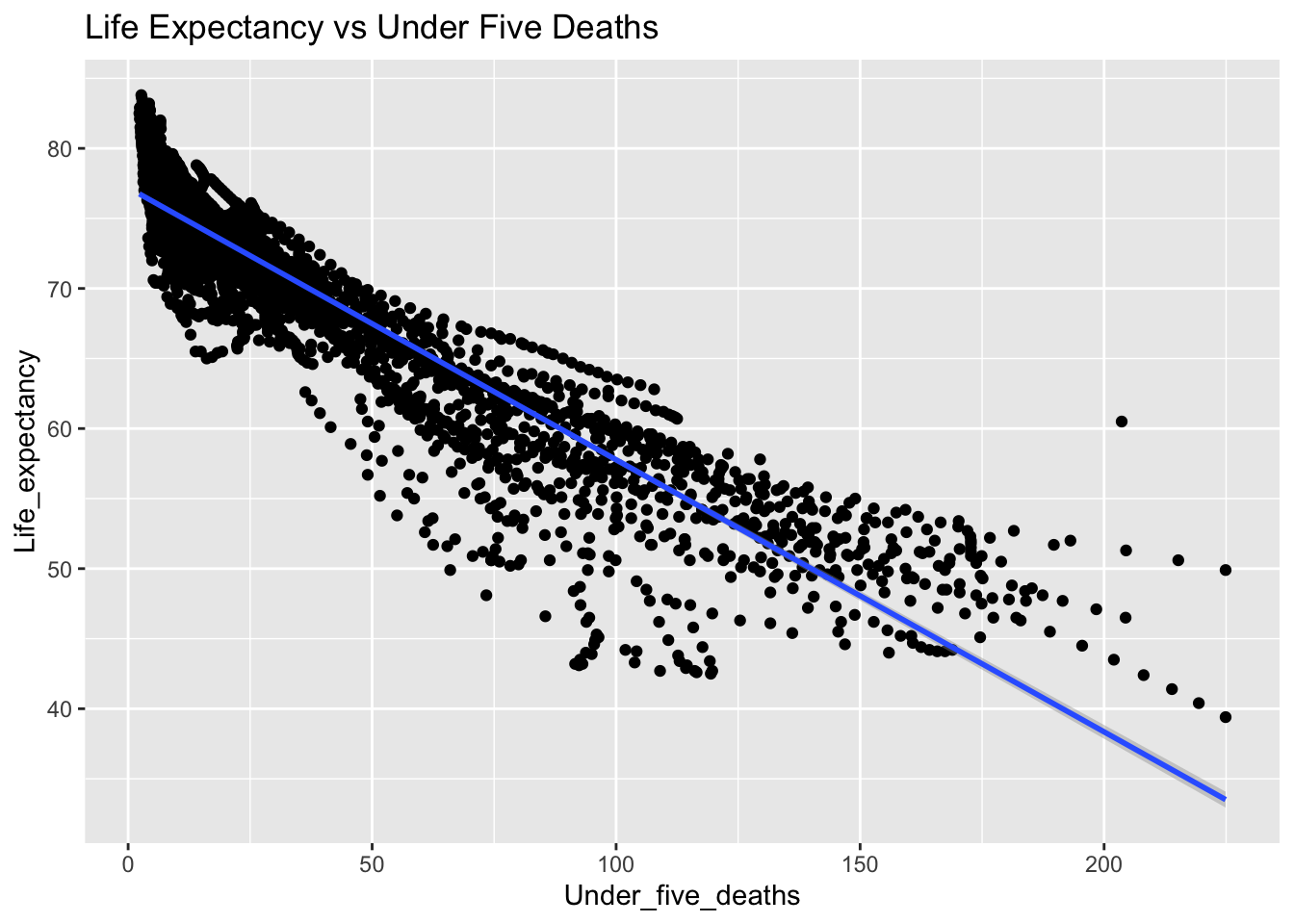

# Scatter plot for Adult_mortality
ggplot(df, aes(x = Adult_mortality, y = Life_expectancy)) +
  geom_point() +               
  geom_smooth(method = "lm") +
  labs(title = "Life Expectancy vs Adult Mortality")

`geom_smooth()` using formula = 'y ~ x'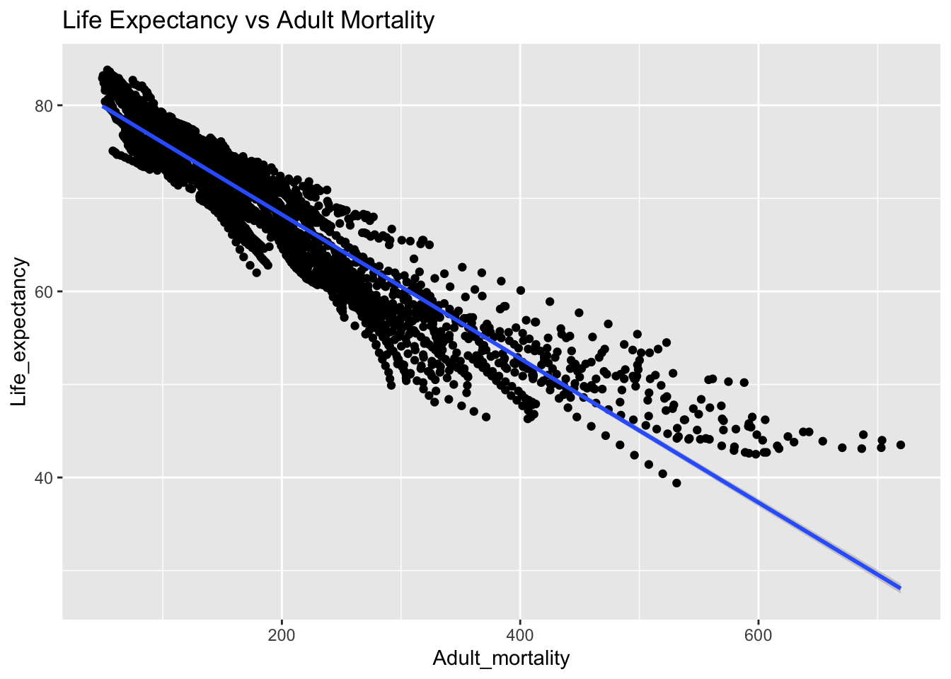

# Scatter plot for Alcohol_consumption
ggplot(df, aes(x = Alcohol_consumption, y = Life_expectancy)) +
  geom_point() +              
  geom_smooth(method = "lm") + 
  labs(title = "Life Expectancy vs Alcohol Consumption")

`geom_smooth()` using formula = 'y ~ x'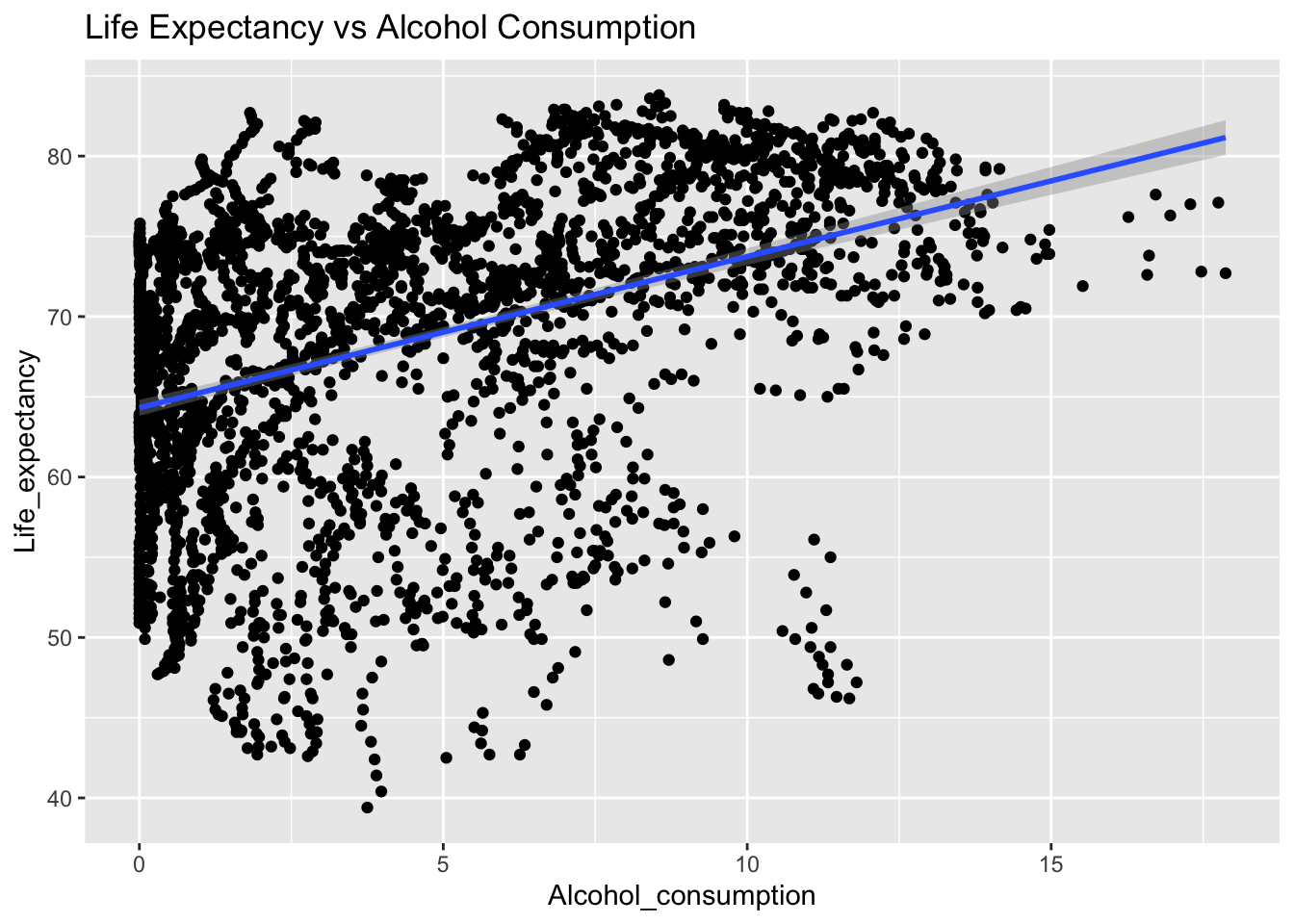

# Scatter plot for BMI
ggplot(df, aes(x = BMI, y = Life_expectancy)) +
  geom_point() +              
  geom_smooth(method = "lm") + 
  labs(title = "Life Expectancy vs BMI")

`geom_smooth()` using formula = 'y ~ x'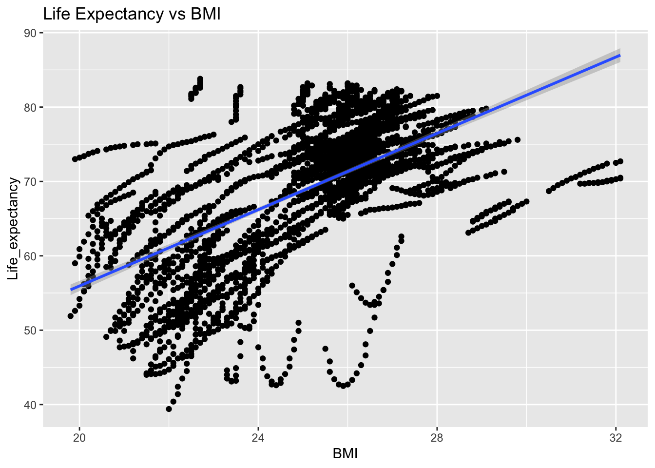

# Scatter plot for Incidents_HIV
ggplot(df, aes(x = Incidents_HIV, y = Life_expectancy)) +
  geom_point() +               
  geom_smooth(method = "lm") + 
  labs(title = "Life Expectancy vs Incidents HIV")

`geom_smooth()` using formula = 'y ~ x'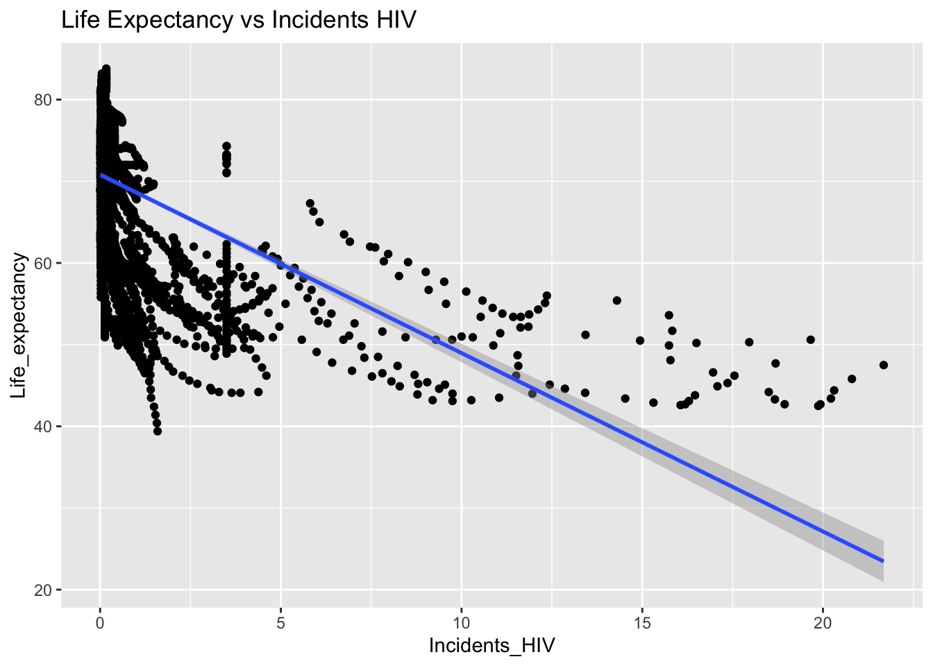

# Scatter plot for GDP_per_capita
ggplot(df, aes(x = GDP_per_capita, y = Life_expectancy)) +
  geom_point() +               
  geom_smooth(method = "lm") + 
  labs(title = "Life Expectancy vs GDP per Capita")

`geom_smooth()` using formula = 'y ~ x'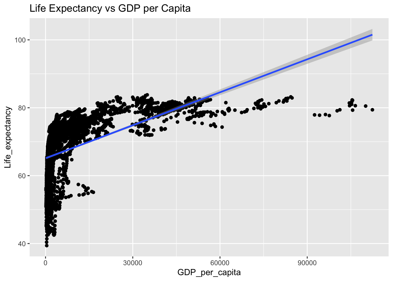

# Scatter plot for Thinness_ten_nineteen_years
ggplot(df, aes(x = Thinness_ten_nineteen_years, y = Life_expectancy)) +
  geom_point() +               
  geom_smooth(method = "lm") + 
  labs(title = "Life Expectancy vs Thinness (10-19 years)")

`geom_smooth()` using formula = 'y ~ x'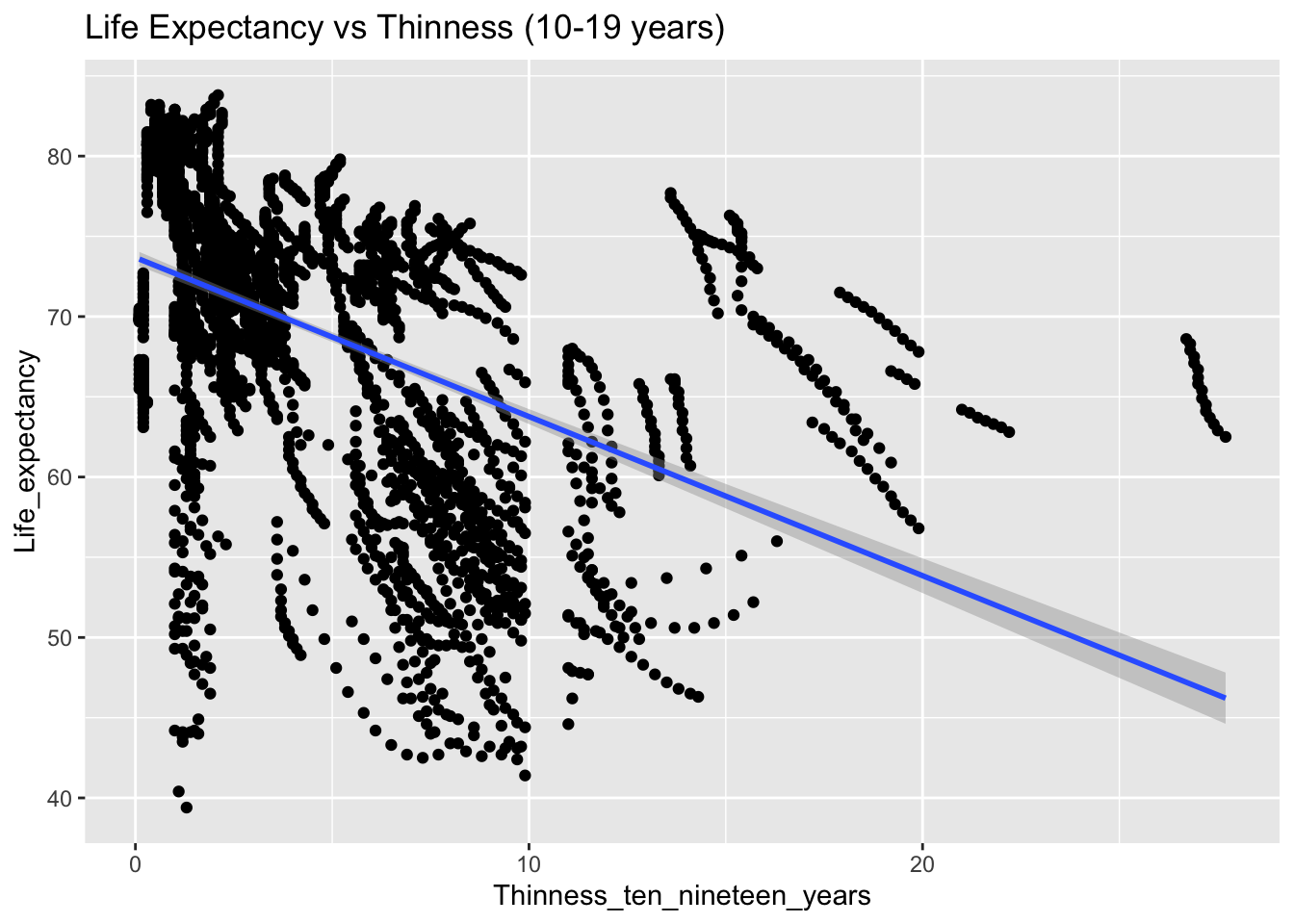

# Scatter plot for Schooling
ggplot(df, aes(x = Schooling, y = Life_expectancy)) +
  geom_point() +              
  geom_smooth(method = "lm") + 
  labs(title = "Life Expectancy vs Schooling")

`geom_smooth()` using formula = 'y ~ x'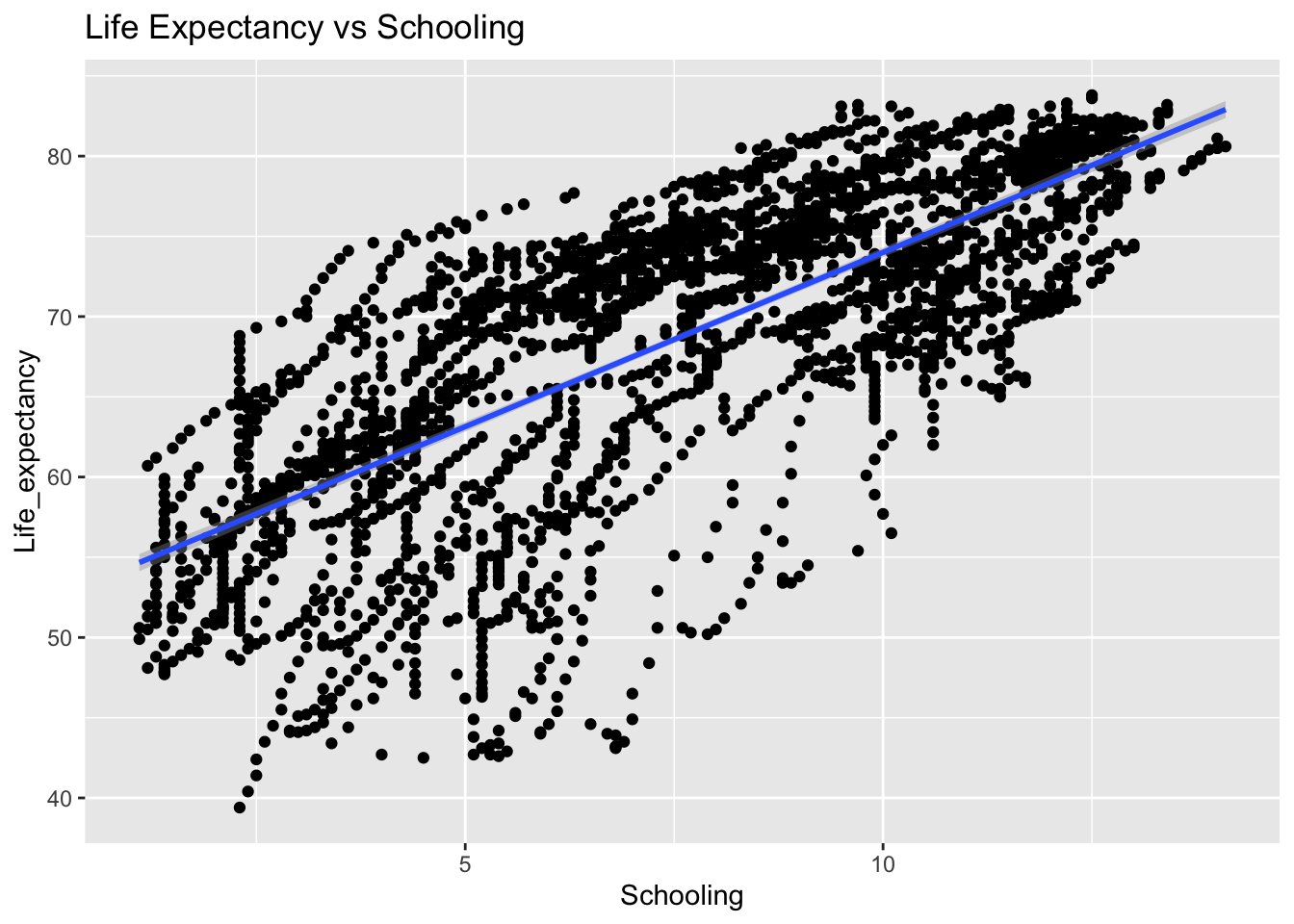

Testing the data

predictions <- predict(LE_MR, newdata = test.data)

rmse <- sqrt(mean(test.data$Life_expectancy - predictions)^2)
print("RMSE 1")

[1] "RMSE 1"

rmse

[1] 0.0006730005

predictions <- predict(LE_MR2, newdata = test.data)

rmse <- sqrt(mean(test.data$Life_expectancy - predictions)^2)
print("RMSE 2")

[1] "RMSE 2"

rmse

[1] 0.006045691

rmsepredictions <- predict(LE_MR3, newdata = test.data)

rmse <- sqrt(mean(test.data$Life_expectancy - predictions)^2)
print("RMSE 3")

[1] "RMSE 3"

rmse

[1] 0.006045691

predictions <- predict(LE_MR4, newdata = test.data)

rmse <- sqrt(mean(test.data$Life_expectancy - predictions)^2)
print("RMSE 4")

[1] "RMSE 4"

rmse

[1] 0.006292047

predictions <- predict(LE_MR5, newdata = test.data)

rmse <- sqrt(mean(test.data$Life_expectancy - predictions)^2)
print("RMSE 5")

[1] "RMSE 5"

rmse

[1] 0.006712114

predictions <- predict(LE_MR6, newdata = test.data)

rmse <- sqrt(mean(test.data$Life_expectancy - predictions)^2)
print("RMSE 6")

[1] "RMSE 6"

rmse

[1] 0.007220434

Comparing the Regression Models
Model	RMSE	Adjusted R^2
LE_MR	0.0006730005	0.9838
LE_MR2	0.006045691	0.9785
LE_MR3	0.006045691	0.9785
LE_MR4	0.006292047	0.9785
LE_MR5	0.006712114	0.9784
LE_MR6	0.007220434	0.9784

5.2 Neural Network of Life Expectancy

Splitting the dataset

glimpse(sdf)

Rows: 2,864
Columns: 21
$ Country                     <fct> "Turkiye", "Spain", "India", "Guyana", "Is…
$ Region                      <fct> Middle East, European Union, Asia, South A…
$ Infant_deaths               <dbl[,1]> <matrix[26 x 1]>
$ Under_five_deaths           <dbl[,1]> <matrix[26 x 1]>
$ Adult_mortality             <dbl[,1]> <matrix[26 x 1]>
$ Alcohol_consumption         <dbl[,1]> <matrix[26 x 1]>
$ Hepatitis_B                 <dbl[,1]> <matrix[26 x 1]>
$ Measles                     <dbl[,1]> <matrix[26 x 1]>
$ BMI                         <dbl[,1]> <matrix[26 x 1]>
$ Polio                       <dbl[,1]> <matrix[26 x 1]>
$ Diphtheria                  <dbl[,1]> <matrix[26 x 1]>
$ Incidents_HIV               <dbl[,1]> <matrix[26 x 1]>
$ GDP_per_capita              <dbl[,1]> <matrix[26 x 1]>
$ Population_mln              <dbl[,1]> <matrix[26 x 1]>
$ Thinness_ten_nineteen_years <dbl[,1]> <matrix[26 x 1]>
$ Thinness_five_nine_years    <dbl[,1]> <matrix[26 x 1]>
$ Schooling                   <dbl[,1]> <matrix[26 x 1]>
$ Economy_status_Developed    <fct> 0, 1, 0, 0, 1, 0, 0, 1, 0, 0, 0, 1, 0,…
$ Economy_status_Developing   <fct> 1, 0, 1, 1, 0, 1, 1, 0, 1, 1, 1, 0, 1,…
$ Life_expectancy             <dbl[,1]> <matrix[26 x 1]>
$ Year                        <fct> 2015, 2015, 2007, 2006, 2012, 2006, 20…

sdf_num <- sdf %>% select_if(is.numeric)

#seed to make this reproducible 
set.seed(444)

#split the data
training.samples. <- sdf$Life_expectancy |> createDataPartition(p = 0.8, list = FALSE)

train_data_nn <- sdf_num[training.samples, ]
test_data_nn <- sdf_num[-training.samples, ]

Training

# Train the neural network
nn <- neuralnet(Life_expectancy ~ . -Diphtheria  - Infant_deaths - Thinness_ten_nineteen_years 
, data = train_data_nn, hidden = 3,
 linear.output = FALSE)
plot(nn)

5.3 SVR model for Life Expectancy

#seed to make this reproducible 
set.seed(444)

#split the data
training.samples <- sdf$Life_expectancy |> createDataPartition(p = 0.8, list = FALSE)

train.data.svm <- sdf[training.samples, ]
test.data.svm <- sdf[-training.samples, ]

The data needs to be scaled for SVR

# Filter out non-numeric columns
numeric_cols <- sapply(train.data.svm, is.numeric)
train.data.svm_numeric <- train.data.svm[, numeric_cols]

# Scale the numeric features
train.data.svm_scaled <- as.data.frame(scale(train.data.svm_numeric))

# Train the SVR model 
LE_SVR <- svm(Life_expectancy ~ . , data = train.data.svm_scaled)

Evaluate Model function:

evaluate_SVR_model <- function(model, test_data) {
  
  actual_values <- test_data$Life_expectancy
  
  # Predict 
  predicted_values <- predict(model, newdata = test_data)
  
  # Calculate evaluation metrics
  mae <- mean(abs(predicted_values - actual_values))
  mse <- mean((predicted_values - actual_values)^2)
  rmse <- sqrt(mse)
  r_squared <- cor(predicted_values, actual_values)^2
  
  # Calculate Adjusted R-squared
  n <- length(actual_values)
  p <- 1  # Assuming you have one predictor, adjust accordingly if you have more
  adjusted_r_squared <- 1 - ((1 - r_squared) * (n - 1) / (n - p - 1))
  
  # Print evaluation metrics
  cat("Mean Absolute Error (MAE):", mae, "\n")
  cat("Mean Squared Error (MSE):", mse, "\n")
  cat("Root Mean Squared Error (RMSE):", rmse, "\n")
  cat("R-squared:", r_squared, "\n")
  cat("Adjusted R-squared:", adjusted_r_squared, "\n")
}

Use the function to evaluate the model

evaluate_SVR_model(LE_SVR, test.data.svm)

Mean Absolute Error (MAE): 0.07397218 
Mean Squared Error (MSE): 0.007783215 
Root Mean Squared Error (RMSE): 0.08822253 
R-squared: 0.9925463 
Adjusted R-squared: 0.9925332

To establish which of the variables are significant we will be removing them one at a time and re-evaluate to see if the model is more or less accurate, Paying attention to the Adjusted R-Square and RMSE especially.

Recursive Feature Elimination - Run this at your own risk!

# Adjust cross-validation settings
# ctrl <- rfeControl(method = "cv", number = 5, verbose = FALSE)

# Use parallel processing

# cores <- parallel::detectCores()
# cl <- makeCluster(cores - 1)  # Use one less core to avoid overloading
# registerDoParallel(cl)

# Perform RFE with scaled features
# rfe_result <- rfe(x = train.data.svm_scaled, 
#                  y = train.data.svm$Life_expectancy,
#                  sizes = c(1:length(predictors)), rfeControl = ctrl)

# Stop parallel processing
# stopCluster(cl)

As RFE is not working for the group, we are going to just brute force it by removing attributes one at a time and see if the models numbers get better.

Glimpse of the data just for checking the names

glimpse(train.data.svm_scaled)

Rows: 2,293
Columns: 16
$ Infant_deaths               <dbl> 0.7590492, 0.0841529, -0.7856332, -0.30562…
$ Under_five_deaths           <dbl> 0.55258540, -0.05825996, -0.73598621, -0.3…
$ Adult_mortality             <dbl> 0.077338858, 0.261532302, 0.006631077, -0.…
$ Alcohol_consumption         <dbl> -0.82494784, 0.20916759, 1.85721042, -1.08…
$ Hepatitis_B                 <dbl> -1.51935470, 0.53879157, 0.22695123, 0.788…
$ Measles                     <dbl> -2.31877381, -0.19600053, 1.16475158, 0.51…
$ BMI                         <dbl> -1.75692499, 0.11855802, 0.39301895, 1.307…
$ Polio                       <dbl> -1.2747616, 0.3605905, 0.8184891, 0.687660…
$ Diphtheria                  <dbl> -1.4035975, 0.4296643, 0.8089598, 0.808959…
$ Incidents_HIV               <dbl> -0.32326406, -0.04478948, -0.34436062, -0.…
$ GDP_per_capita              <dbl> -0.6173467, -0.4339117, -0.1456139, -0.460…
$ Population_mln              <dbl> 7.79008710, -0.26103660, -0.19662543, -0.2…
$ Thinness_ten_nineteen_years <dbl> 4.9415722, 0.1836360, -0.5722978, -0.19433…
$ Thinness_five_nine_years    <dbl> 5.0464300, 0.1296280, -0.5696505, -0.22001…
$ Schooling                   <dbl> -0.83048406, 0.08144663, 0.80470200, 0.616…
$ Life_expectancy             <dbl> -0.36755454, -0.19705890, 0.25049214, 0.32…

#Without Infant_deaths
LE_SVR_Testing <- svm(Life_expectancy ~ . - Infant_deaths, data = train.data.svm_scaled)

evaluate_SVR_model(LE_SVR_Testing, test.data.svm)

Mean Absolute Error (MAE): 0.07471295 
Mean Squared Error (MSE): 0.007852998 
Root Mean Squared Error (RMSE): 0.08861714 
R-squared: 0.9924428 
Adjusted R-squared: 0.9924295

#Without Under_five_deaths
LE_SVR_Testing <- svm(Life_expectancy ~ . - Under_five_deaths, data = train.data.svm_scaled)

evaluate_SVR_model(LE_SVR_Testing, test.data.svm)

Mean Absolute Error (MAE): 0.07619821 
Mean Squared Error (MSE): 0.008231436 
Root Mean Squared Error (RMSE): 0.09072726 
R-squared: 0.9920679 
Adjusted R-squared: 0.992054

#Adult_mortality
LE_SVR_Testing <- svm(Life_expectancy ~ . - Adult_mortality, data = train.data.svm_scaled)

evaluate_SVR_model(LE_SVR_Testing, test.data.svm)

Mean Absolute Error (MAE): 0.1133804 
Mean Squared Error (MSE): 0.02399256 
Root Mean Squared Error (RMSE): 0.1548953 
R-squared: 0.9766539 
Adjusted R-squared: 0.9766129

#Alcohol_consumption
LE_SVR_Testing<- svm(Life_expectancy ~ . - Alcohol_consumption, data = train.data.svm_scaled)

evaluate_SVR_model(LE_SVR_Testing, test.data.svm)

Mean Absolute Error (MAE): 0.07744333 
Mean Squared Error (MSE): 0.008586509 
Root Mean Squared Error (RMSE): 0.09266342 
R-squared: 0.9916855 
Adjusted R-squared: 0.9916709

#Hepatitis_B                 
LE_SVR_Testing<- svm(Life_expectancy ~ . - Hepatitis_B                 , data = train.data.svm_scaled)

evaluate_SVR_model(LE_SVR_Testing, test.data.svm)

Mean Absolute Error (MAE): 0.07241759 
Mean Squared Error (MSE): 0.007626557 
Root Mean Squared Error (RMSE): 0.08733016 
R-squared: 0.9926655 
Adjusted R-squared: 0.9926526

#Measles                                      
LE_SVR_Testing<- svm(Life_expectancy ~ . - Measles, data = train.data.svm_scaled)

evaluate_SVR_model(LE_SVR_Testing, test.data.svm)

Mean Absolute Error (MAE): 0.07528426 
Mean Squared Error (MSE): 0.008338268 
Root Mean Squared Error (RMSE): 0.09131412 
R-squared: 0.9919717 
Adjusted R-squared: 0.9919576

#BMI                                      
LE_SVR_Testing<- svm(Life_expectancy ~ . - BMI, data = train.data.svm_scaled)

evaluate_SVR_model(LE_SVR_Testing, test.data.svm)

Mean Absolute Error (MAE): 0.07787055 
Mean Squared Error (MSE): 0.009170201 
Root Mean Squared Error (RMSE): 0.09576117 
R-squared: 0.9912598 
Adjusted R-squared: 0.9912444

#Polio                                      
LE_SVR_Testing<- svm(Life_expectancy ~ . - Polio, data = train.data.svm_scaled)

evaluate_SVR_model(LE_SVR_Testing, test.data.svm)

Mean Absolute Error (MAE): 0.07443335 
Mean Squared Error (MSE): 0.007857034 
Root Mean Squared Error (RMSE): 0.08863991 
R-squared: 0.9925017 
Adjusted R-squared: 0.9924885

#Diphtheria                                     
LE_SVR_Testing<- svm(Life_expectancy ~ . - Diphtheria, data = train.data.svm_scaled)

evaluate_SVR_model(LE_SVR_Testing, test.data.svm)

Mean Absolute Error (MAE): 0.07355648 
Mean Squared Error (MSE): 0.007704026 
Root Mean Squared Error (RMSE): 0.08777258 
R-squared: 0.9926214 
Adjusted R-squared: 0.9926085

#Incidents_HIV                                     
LE_SVR_Testing<- svm(Life_expectancy ~ . - Incidents_HIV, data = train.data.svm_scaled)

evaluate_SVR_model(LE_SVR_Testing, test.data.svm)

Mean Absolute Error (MAE): 0.07527161 
Mean Squared Error (MSE): 0.008397796 
Root Mean Squared Error (RMSE): 0.09163949 
R-squared: 0.9918974 
Adjusted R-squared: 0.9918832

#GDP_per_capita                                     
LE_SVR_Testing<- svm(Life_expectancy ~ . - GDP_per_capita, data = train.data.svm_scaled)

evaluate_SVR_model(LE_SVR_Testing, test.data.svm)

Mean Absolute Error (MAE): 0.07584458 
Mean Squared Error (MSE): 0.008198734 
Root Mean Squared Error (RMSE): 0.09054686 
R-squared: 0.9921686 
Adjusted R-squared: 0.9921549

#Population_mln                                     
LE_SVR_Testing<- svm(Life_expectancy ~ . - Population_mln, data = train.data.svm_scaled)

evaluate_SVR_model(LE_SVR_Testing, test.data.svm)

Mean Absolute Error (MAE): 0.07505001 
Mean Squared Error (MSE): 0.008137925 
Root Mean Squared Error (RMSE): 0.09021045 
R-squared: 0.992191 
Adjusted R-squared: 0.9921773

#Thinness_ten_nineteen_years
LE_SVR_Testing<- svm(Life_expectancy ~ . - Thinness_ten_nineteen_years, data = train.data.svm_scaled)

evaluate_SVR_model(LE_SVR_Testing, test.data.svm)

Mean Absolute Error (MAE): 0.07369326 
Mean Squared Error (MSE): 0.007717285 
Root Mean Squared Error (RMSE): 0.08784808 
R-squared: 0.9925828 
Adjusted R-squared: 0.9925698

#Thinness_five_nine_years
LE_SVR_Testing<- svm(Life_expectancy ~ . - Thinness_five_nine_years, data = train.data.svm_scaled)

evaluate_SVR_model(LE_SVR_Testing, test.data.svm)

Mean Absolute Error (MAE): 0.07403657 
Mean Squared Error (MSE): 0.007772499 
Root Mean Squared Error (RMSE): 0.08816178 
R-squared: 0.9925884 
Adjusted R-squared: 0.9925753

#Schooling
LE_SVR_Testing<- svm(Life_expectancy ~ . - Schooling, data = train.data.svm_scaled)

evaluate_SVR_model(LE_SVR_Testing, test.data.svm)

Mean Absolute Error (MAE): 0.07663966 
Mean Squared Error (MSE): 0.008466487 
Root Mean Squared Error (RMSE): 0.09201351 
R-squared: 0.9918468 
Adjusted R-squared: 0.9918324

Table comparing the different SVR models.

Removed Variable	MAE	MSE	RMSE	R-Squared	Adjusted R-Squared
None (Base)	0.07395971	0.00778042	0.08820669	0.9925481	0.992535
Infant deaths	0.07470623	0.007850003	0.08860024	0.992445	0.9924317
Under five deaths	0.07621305	0.008232278	0.0907319	0.9920679	0.992054
Adult mortality	0.1133804	0.02399256	0.1548953	0.9766539	0.9766129
Alcohol consumption	0.07744333	0.008586509	0.09266342	0.9916855	0.9916709
Hepatitis B	0.07243036	0.007626723	0.08733111	0.992664	0.9926511
Measles	0.07528426	0.008338268	0.09131412	0.9919717	0.9919576
BMI	0.07787055	0.009170201	0.09576117	0.9912598	0.9912444
Polio	0.0744371	0.007858702	0.08864932	0.9925011	0.9924879
Diphtheria	0.07355422	0.007703352	0.08776874	0.9926202	0.9926072
Incidents HIV	0.07527161	0.008397796	0.09163949	0.9918974	0.9918832
GDP per capita	0.07584458	0.008198734	0.09054686	0.9921686	0.9921549
Population mln	0.07505001	0.008137925	0.09021045	0.992191	0.9921773
Thinness ten nineteen years	0.07371203	0.007720199	0.08786466	0.992582	0.992569
Thinness five nine years	0.0740283	0.007773223	0.08816589	0.9925873	0.9925743
Schooling	0.07663966	0.008466487	0.09201351	0.9918468	0.9918324

The general idea of this table is that the worse the model does without the given variable, the more important the variable is to the SVR model.

The fact that Infant deaths and Under 5 deaths are not showing as significant is interesting, as every other model shows them as being very significant. It is possible that due to the Multicollinearity between them, removing one will not have much of an effect as the other is still present in the model, to test this we will remove both to see what happens.

LE_SVR_Testing<- svm(Life_expectancy ~ . - Under_five_deaths -Infant_deaths, data = train.data.svm_scaled)

evaluate_SVR_model(LE_SVR_Testing, test.data.svm)

Mean Absolute Error (MAE): 0.08451521 
Mean Squared Error (MSE): 0.01103041 
Root Mean Squared Error (RMSE): 0.1050258 
R-squared: 0.989295 
Adjusted R-squared: 0.9892762

And yes, this is having a very large effect on the model, its not perfectly comparable to the removal of one of the variables at a time, but it is enough for us to assume that Infant Deaths and Under five deaths are more significant that the table initially lets on.

5.3.1 Conclusion of SVR Model

Adult_Mortality, BMI and Schooling all negatively impact the model enough when removed to be significant.

This method is not without it faults however, as it doesn’t identify Under_five_deaths or Infant_deaths as significant. However if both are removed from the model, it causes a significant increase in error of the model. As we laid out in the previous model, these variables are high in multicollinearity. It is very possible that the removal of one of these is beneficial to the model, to prevent over-fitting, and the negative effects of removing these significant attributes is only shown when both are removed.

5.4 Random Forest

Set up the data for Random Forest:

RF_DF <- df[, !(names(df) %in% c("Region", "Country", "Economy_status_Developed", "Economy_status_Developing","Year"))]

summary(RF_DF)

 Infant_deaths    Under_five_deaths Adult_mortality  Alcohol_consumption
 Min.   :  1.80   Min.   :  2.300   Min.   : 49.38   Min.   : 0.000     
 1st Qu.:  8.10   1st Qu.:  9.675   1st Qu.:106.91   1st Qu.: 1.200     
 Median : 19.60   Median : 23.100   Median :163.84   Median : 4.020     
 Mean   : 30.36   Mean   : 42.938   Mean   :192.25   Mean   : 4.821     
 3rd Qu.: 47.35   3rd Qu.: 66.000   3rd Qu.:246.79   3rd Qu.: 7.777     
 Max.   :138.10   Max.   :224.900   Max.   :719.36   Max.   :17.870     
  Hepatitis_B       Measles           BMI            Polio        Diphtheria   
 Min.   :12.00   Min.   :10.00   Min.   :19.80   Min.   : 8.0   Min.   :16.00  
 1st Qu.:78.00   1st Qu.:64.00   1st Qu.:23.20   1st Qu.:81.0   1st Qu.:81.00  
 Median :89.00   Median :83.00   Median :25.50   Median :93.0   Median :93.00  
 Mean   :84.29   Mean   :77.34   Mean   :25.03   Mean   :86.5   Mean   :86.27  
 3rd Qu.:96.00   3rd Qu.:93.00   3rd Qu.:26.40   3rd Qu.:97.0   3rd Qu.:97.00  
 Max.   :99.00   Max.   :99.00   Max.   :32.10   Max.   :99.0   Max.   :99.00  
 Incidents_HIV     GDP_per_capita   Population_mln    
 Min.   : 0.0100   Min.   :   148   Min.   :   0.080  
 1st Qu.: 0.0800   1st Qu.:  1416   1st Qu.:   2.098  
 Median : 0.1500   Median :  4217   Median :   7.850  
 Mean   : 0.8943   Mean   : 11541   Mean   :  36.676  
 3rd Qu.: 0.4600   3rd Qu.: 12557   3rd Qu.:  23.688  
 Max.   :21.6800   Max.   :112418   Max.   :1379.860  
 Thinness_ten_nineteen_years Thinness_five_nine_years   Schooling     
 Min.   : 0.100              Min.   : 0.1             Min.   : 1.100  
 1st Qu.: 1.600              1st Qu.: 1.6             1st Qu.: 5.100  
 Median : 3.300              Median : 3.4             Median : 7.800  
 Mean   : 4.866              Mean   : 4.9             Mean   : 7.632  
 3rd Qu.: 7.200              3rd Qu.: 7.3             3rd Qu.:10.300  
 Max.   :27.700              Max.   :28.6             Max.   :14.100  
 Life_expectancy
 Min.   :39.40  
 1st Qu.:62.70  
 Median :71.40  
 Mean   :68.86  
 3rd Qu.:75.40  
 Max.   :83.80

Split the data:

# Set seed for reproducibility
set.seed(321)

# Split the data into training and testing sets
train_index_RF <- createDataPartition(RF_DF$Life_expectancy, p = 0.8, list = FALSE)
train_data_RF <- RF_DF[train_index_RF, ]
test_data_RF <- RF_DF[-train_index_RF, ]

Making the model:

# Train the random forest model
rf_model <- randomForest(Life_expectancy ~ ., data = train_data_RF, ntree = 500)

# Print the trained model
print(rf_model)


Call:
 randomForest(formula = Life_expectancy ~ ., data = train_data_RF,      ntree = 500) 
               Type of random forest: regression
                     Number of trees: 500
No. of variables tried at each split: 5

          Mean of squared residuals: 0.2893711
                    % Var explained: 99.67

Assessing the model:

predicted_values <- predict(rf_model, test_data_RF)

rmse_value <- sqrt(mean((predicted_values - test_data_RF$Life_expectancy)^2))
print(paste("RMSE:", rmse_value))

[1] "RMSE: 0.499788784239889"

# R-squared
observed_values <- test_data_RF$Life_expectancy
r_squared <- cor(observed_values, predicted_values)^2
print(paste("R-squared:", r_squared))

[1] "R-squared: 0.997343879005976"

Significance plot:

# Print variable importance
print(rf_model$importance)

                            IncNodePurity
Infant_deaths                  38309.0795
Under_five_deaths              62636.1320
Adult_mortality                51316.8181
Alcohol_consumption             1260.6709
Hepatitis_B                      330.7512
Measles                         1600.2814
BMI                             5418.3906
Polio                           1192.1789
Diphtheria                       770.9613
Incidents_HIV                  16695.6777
GDP_per_capita                 10782.2387
Population_mln                   848.2376
Thinness_ten_nineteen_years     1139.3053
Thinness_five_nine_years        1346.8517
Schooling                       7127.5208

This gives us another way to answer to see which variables are significant for Life Expectancy.

Interpreting these values:

Infant_deaths, Under_five_deaths, and Adult_mortality have the highest importance scores, indicating that they are the most important predictors of life expectancy in your model.
Alcohol_consumption, BMI, Incidents_HIV, GDP_per_capita, and Schooling also have relatively high importance scores, suggesting that they significantly contribute to the model’s predictive performance.
Hepatitis_B, Measles, Polio, Diphtheria, Population_mln, Thinness_ten_nineteen_years, and Thinness_five_nine_years have relatively less impact on the model compared to others.

This backs up the Multiple Regression model findings.

5.5 Which Variables Most Influence Life Expectancy

From the various model made above, it seems conclusive that the most significant variables for Life Expectancy are Infant_deaths, Under_five_deaths, and Adult_mortality. This is not a surprising conclusion as all three of these variables directly relate to death at a certain age, which is what Life Expectancy is measuring.

The more interesting variables of significance are Alcohol_consumption, BMI, Incidents_HIV, GDP_per_capita, and Schooling.

Incidents of HIV is again no surprise as HIV is a debilitating illness that if untreated will result in death, therefore the higher the rate of HIV the lower the life expectancy.

The other variables in this group are more interesting, and seem to correlate with a nation being more developed, and thus having more access to healthcare, and thus a higher life expectancy.

5.6 Comparing the Models

For each of these models if multiple models were made, we are using the final version of the model for comparison.

Model	RMSE	Adjusted R^2
Multiple Regression	0.007220434	0.9784
Random Forest	0.5001062729781	0.9973385774022
SVR	0.08820669	0.992533

According to these numbers, the Multiple Regression model is the most accurate.

5.7 Predict Countries Economic Status from Life Expectancy

5.7.1 Logistic Regression Model

glimpse(df)

Rows: 2,864
Columns: 21
$ Country                     <fct> "Turkiye", "Spain", "India", "Guyana", "Is…
$ Region                      <fct> Middle East, European Union, Asia, South A…
$ Year                        <fct> 2015, 2015, 2007, 2006, 2012, 2006, 2015, …
$ Infant_deaths               <dbl> 11.1, 2.7, 51.5, 32.8, 3.4, 9.8, 6.6, 8.7,…
$ Under_five_deaths           <dbl> 13.0, 3.3, 67.9, 40.5, 4.3, 11.2, 8.2, 10.…
$ Adult_mortality             <dbl> 105.8240, 57.9025, 201.0765, 222.1965, 57.…
$ Alcohol_consumption         <dbl> 1.32, 10.35, 1.57, 5.68, 2.89, 4.19, 8.06,…
$ Hepatitis_B                 <dbl> 97, 97, 60, 93, 97, 88, 97, 88, 97, 97, 96…
$ Measles                     <dbl> 65, 94, 35, 74, 89, 86, 97, 99, 87, 92, 70…
$ BMI                         <dbl> 27.8, 26.0, 21.2, 25.3, 27.0, 26.4, 26.2, …
$ Polio                       <dbl> 97, 97, 67, 92, 94, 89, 97, 99, 97, 96, 96…
$ Diphtheria                  <dbl> 97, 97, 64, 93, 94, 89, 97, 99, 99, 90, 95…
$ Incidents_HIV               <dbl> 0.08, 0.09, 0.13, 0.79, 0.08, 0.16, 0.08, …
$ GDP_per_capita              <dbl> 11006, 25742, 1076, 4146, 33995, 9110, 931…
$ Population_mln              <dbl> 78.53, 46.44, 1183.21, 0.75, 7.91, 4.35, 1…
$ Thinness_ten_nineteen_years <dbl> 4.9, 0.6, 27.1, 5.7, 1.2, 2.0, 2.3, 2.3, 4…
$ Thinness_five_nine_years    <dbl> 4.8, 0.5, 28.0, 5.5, 1.1, 1.9, 2.3, 2.3, 3…
$ Schooling                   <dbl> 7.8, 9.7, 5.0, 7.9, 12.8, 7.9, 12.0, 10.2,…
$ Economy_status_Developed    <fct> 0, 1, 0, 0, 1, 0, 0, 1, 0, 0, 0, 1, 0, 0, …
$ Economy_status_Developing   <fct> 1, 0, 1, 1, 0, 1, 1, 0, 1, 1, 1, 0, 1, 1, …
$ Life_expectancy             <dbl> 76.5, 82.8, 65.4, 67.0, 81.7, 78.2, 71.2, …

split the data

set.seed(17)

partition_index <- createDataPartition(df$Economy_status_Developed, p = 0.7, list = FALSE)

train_data_log <- df[partition_index,]
validation_data_log <- df[-partition_index,]

make the model

LE_Log <- glm(Economy_status_Developed ~ Life_expectancy,
              data = train_data_log,
              family = binomial)

Summary of the model:

summary(LE_Log)


Call:
glm(formula = Economy_status_Developed ~ Life_expectancy, family = binomial, 
    data = train_data_log)

Coefficients:
                 Estimate Std. Error z value Pr(>|z|)    
(Intercept)     -41.61314    2.17086  -19.17   <2e-16 ***
Life_expectancy   0.53984    0.02848   18.95   <2e-16 ***
---
Signif. codes:  0 '***' 0.001 '**' 0.01 '*' 0.05 '.' 0.1 ' ' 1

(Dispersion parameter for binomial family taken to be 1)

    Null deviance: 2045.29  on 2005  degrees of freedom
Residual deviance:  965.27  on 2004  degrees of freedom
AIC: 969.27

Number of Fisher Scoring iterations: 7

As expected from our previous question, Life Expectancy is significant to the countries status, with a P Value of 2e-16.

Odds Ratio

odds_ratio <- exp(coef(LE_Log))

print(odds_ratio)

    (Intercept) Life_expectancy 
   8.465307e-19    1.715740e+00

Predictions and Confusion matrix

predictions <- predict(LE_Log, validation_data_log, type = "response" )

binary_predictions <- ifelse(predictions > 0.5, 1, 0)

confusion_Matrix <- confusionMatrix(factor(binary_predictions), factor(validation_data_log$Economy_status_Developed))

print(confusion_Matrix)

Confusion Matrix and Statistics

          Reference
Prediction   0   1
         0 639  45
         1  42 132
                                         
               Accuracy : 0.8986         
                 95% CI : (0.8764, 0.918)
    No Information Rate : 0.7937         
    P-Value [Acc > NIR] : <2e-16         
                                         
                  Kappa : 0.6884         
                                         
 Mcnemar's Test P-Value : 0.8302         
                                         
            Sensitivity : 0.9383         
            Specificity : 0.7458         
         Pos Pred Value : 0.9342         
         Neg Pred Value : 0.7586         
             Prevalence : 0.7937         
         Detection Rate : 0.7448         
   Detection Prevalence : 0.7972         
      Balanced Accuracy : 0.8420         
                                         
       'Positive' Class : 0

Overall accuracy: 90.1%

Specificity: 70.62%

Sensitivity: 95.16%

Overall a very good model, going off this confusion matrix. However can we make it better?

ROC Curve

 la.roc <- roc(validation_data_log$Economy_status_Developed, predictions)

Setting levels: control = 0, case = 1

Setting direction: controls < cases

 plot.roc(la.roc, print.auc = TRUE, print.thres ="best")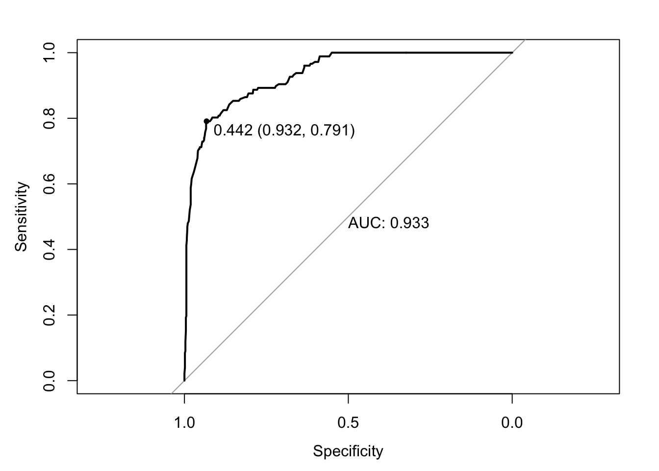

From this we have learned that the best threshold for this model for predictions would be 0.308

Remake the model with the best threshold.

predictions <- predict(LE_Log, validation_data_log, type = "response" )

binary_predictions <- ifelse(predictions > 0.308, 1, 0)

confusion_Matrix <- confusionMatrix(factor(binary_predictions), factor(validation_data_log$Economy_status_Developed))

print(confusion_Matrix)

Confusion Matrix and Statistics

          Reference
Prediction   0   1
         0 608  34
         1  73 143
                                          
               Accuracy : 0.8753          
                 95% CI : (0.8513, 0.8967)
    No Information Rate : 0.7937          
    P-Value [Acc > NIR] : 2.69e-10        
                                          
                  Kappa : 0.6479          
                                          
 Mcnemar's Test P-Value : 0.0002392       
                                          
            Sensitivity : 0.8928          
            Specificity : 0.8079          
         Pos Pred Value : 0.9470          
         Neg Pred Value : 0.6620          
             Prevalence : 0.7937          
         Detection Rate : 0.7086          
   Detection Prevalence : 0.7483          
      Balanced Accuracy : 0.8504          
                                          
       'Positive' Class : 0

Overall accuracy: 89.76%

Specificity: 83.05%

Sensitivity: 91.5%

Please note that this “Best” model is simply the one with the highest sum of sensitivity and specificity. As we do not have any costs associated with false negatives and false positives it is not possible to determine what the best model for our situation is.

5.7.2 XG Boost Model

glimpse(df)

Rows: 2,864
Columns: 21
$ Country                     <fct> "Turkiye", "Spain", "India", "Guyana", "Is…
$ Region                      <fct> Middle East, European Union, Asia, South A…
$ Year                        <fct> 2015, 2015, 2007, 2006, 2012, 2006, 2015, …
$ Infant_deaths               <dbl> 11.1, 2.7, 51.5, 32.8, 3.4, 9.8, 6.6, 8.7,…
$ Under_five_deaths           <dbl> 13.0, 3.3, 67.9, 40.5, 4.3, 11.2, 8.2, 10.…
$ Adult_mortality             <dbl> 105.8240, 57.9025, 201.0765, 222.1965, 57.…
$ Alcohol_consumption         <dbl> 1.32, 10.35, 1.57, 5.68, 2.89, 4.19, 8.06,…
$ Hepatitis_B                 <dbl> 97, 97, 60, 93, 97, 88, 97, 88, 97, 97, 96…
$ Measles                     <dbl> 65, 94, 35, 74, 89, 86, 97, 99, 87, 92, 70…
$ BMI                         <dbl> 27.8, 26.0, 21.2, 25.3, 27.0, 26.4, 26.2, …
$ Polio                       <dbl> 97, 97, 67, 92, 94, 89, 97, 99, 97, 96, 96…
$ Diphtheria                  <dbl> 97, 97, 64, 93, 94, 89, 97, 99, 99, 90, 95…
$ Incidents_HIV               <dbl> 0.08, 0.09, 0.13, 0.79, 0.08, 0.16, 0.08, …
$ GDP_per_capita              <dbl> 11006, 25742, 1076, 4146, 33995, 9110, 931…
$ Population_mln              <dbl> 78.53, 46.44, 1183.21, 0.75, 7.91, 4.35, 1…
$ Thinness_ten_nineteen_years <dbl> 4.9, 0.6, 27.1, 5.7, 1.2, 2.0, 2.3, 2.3, 4…
$ Thinness_five_nine_years    <dbl> 4.8, 0.5, 28.0, 5.5, 1.1, 1.9, 2.3, 2.3, 3…
$ Schooling                   <dbl> 7.8, 9.7, 5.0, 7.9, 12.8, 7.9, 12.0, 10.2,…
$ Economy_status_Developed    <fct> 0, 1, 0, 0, 1, 0, 0, 1, 0, 0, 0, 1, 0, 0, …
$ Economy_status_Developing   <fct> 1, 0, 1, 1, 0, 1, 1, 0, 1, 1, 1, 0, 1, 1, …
$ Life_expectancy             <dbl> 76.5, 82.8, 65.4, 67.0, 81.7, 78.2, 71.2, …

Any factors need to be turned back into numeric values for this model:

xgdf <- df %>%
  mutate_if(is.factor, as.numeric)

xgdf <- xgdf %>%
  select(Life_expectancy, Economy_status_Developed)

Split the data:

set.seed(101)

# Create train-test split
train_index <- createDataPartition(xgdf$Economy_status_Developed, p = 0.8, list = FALSE)
train_data <- xgdf[train_index, ]
test_data <- xgdf[-train_index, ]

XGBoost requires a specific format, DMatrix:

# Convert labels to binary format
train_data$Economy_status_Developed <- ifelse(train_data$Economy_status_Developed == 1, 0, 1)

# Train data
dtrain <- xgb.DMatrix(data = as.matrix(train_data[, -ncol(train_data)]), label = train_data$Economy_status_Developed)

# Test data
dtest <- xgb.DMatrix(data = as.matrix(test_data[, -ncol(test_data)]), label = test_data$Economy_status_Developed)

Now we can actually make the model:

params <- list(
  booster = "gbtree",
  objective = "binary:logistic",
  eta = 0.1,
  gamma = 1,
  max_depth = 6,
  min_child_weight = 1,
  subsample = 0.8,
  colsample_bytree = 0.8
)

# Train the model
XG_model <- xgb.train(params = params, data = dtrain, nrounds = 100, watchlist = list(train = dtrain, test = dtest), early_stopping_rounds = 10)

[1] train-logloss:0.625828  test-logloss:0.746798 
Multiple eval metrics are present. Will use test_logloss for early stopping.
Will train until test_logloss hasn't improved in 10 rounds.

[2] train-logloss:0.570548  test-logloss:0.802487 
[3] train-logloss:0.524475  test-logloss:0.858668 
[4] train-logloss:0.485445  test-logloss:0.916790 
[5] train-logloss:0.452155  test-logloss:0.972407 
[6] train-logloss:0.424040  test-logloss:1.029547 
[7] train-logloss:0.400175  test-logloss:1.084337 
[8] train-logloss:0.379408  test-logloss:1.138477 
[9] train-logloss:0.361277  test-logloss:1.194970 
[10]    train-logloss:0.345439  test-logloss:1.251218 
[11]    train-logloss:0.331490  test-logloss:1.304111 
Stopping. Best iteration:
[1] train-logloss:0.625828  test-logloss:0.746798

Predictions and Confusion Matrix:

preds <- predict(XG_model, dtest)

predicted_labels <- ifelse(preds > 0.5, 1, 0)

predicted_labels_factor <- factor(predicted_labels, levels = c(0, 1))
actual_labels_factor <- factor(test_data$Economy_status_Developed, levels = c(0, 1))

# Compute the confusion matrix
conf_matrix <- confusionMatrix(predicted_labels_factor, actual_labels_factor)
print(conf_matrix)

Confusion Matrix and Statistics

          Reference
Prediction   0   1
         0   0 445
         1   0  19
                                          
               Accuracy : 0.0409          
                 95% CI : (0.0248, 0.0632)
    No Information Rate : 1               
    P-Value [Acc > NIR] : 1               
                                          
                  Kappa : 0               
                                          
 Mcnemar's Test P-Value : <2e-16          
                                          
            Sensitivity :      NA         
            Specificity : 0.04095         
         Pos Pred Value :      NA         
         Neg Pred Value :      NA         
             Prevalence : 0.00000         
         Detection Rate : 0.00000         
   Detection Prevalence : 0.95905         
      Balanced Accuracy :      NA         
                                          
       'Positive' Class : 0

Sensitivity: 96.34%

Specificity: 67.59%

Overall Accuracy: 90.90%

 xg.roc <- roc(test_data$Economy_status_Developed, preds)

Setting levels: control = 1, case = 2

Setting direction: controls < cases

 plot.roc(xg.roc, print.auc = TRUE, print.thres ="best")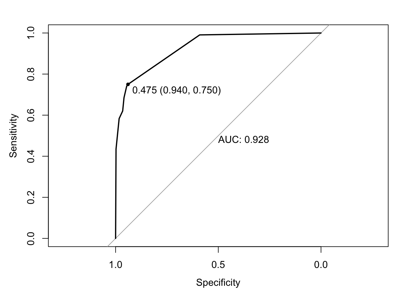

5.7.3 Decision Tree

glimpse(df)

Rows: 2,864
Columns: 21
$ Country                     <fct> "Turkiye", "Spain", "India", "Guyana", "Is…
$ Region                      <fct> Middle East, European Union, Asia, South A…
$ Year                        <fct> 2015, 2015, 2007, 2006, 2012, 2006, 2015, …
$ Infant_deaths               <dbl> 11.1, 2.7, 51.5, 32.8, 3.4, 9.8, 6.6, 8.7,…
$ Under_five_deaths           <dbl> 13.0, 3.3, 67.9, 40.5, 4.3, 11.2, 8.2, 10.…
$ Adult_mortality             <dbl> 105.8240, 57.9025, 201.0765, 222.1965, 57.…
$ Alcohol_consumption         <dbl> 1.32, 10.35, 1.57, 5.68, 2.89, 4.19, 8.06,…
$ Hepatitis_B                 <dbl> 97, 97, 60, 93, 97, 88, 97, 88, 97, 97, 96…
$ Measles                     <dbl> 65, 94, 35, 74, 89, 86, 97, 99, 87, 92, 70…
$ BMI                         <dbl> 27.8, 26.0, 21.2, 25.3, 27.0, 26.4, 26.2, …
$ Polio                       <dbl> 97, 97, 67, 92, 94, 89, 97, 99, 97, 96, 96…
$ Diphtheria                  <dbl> 97, 97, 64, 93, 94, 89, 97, 99, 99, 90, 95…
$ Incidents_HIV               <dbl> 0.08, 0.09, 0.13, 0.79, 0.08, 0.16, 0.08, …
$ GDP_per_capita              <dbl> 11006, 25742, 1076, 4146, 33995, 9110, 931…
$ Population_mln              <dbl> 78.53, 46.44, 1183.21, 0.75, 7.91, 4.35, 1…
$ Thinness_ten_nineteen_years <dbl> 4.9, 0.6, 27.1, 5.7, 1.2, 2.0, 2.3, 2.3, 4…
$ Thinness_five_nine_years    <dbl> 4.8, 0.5, 28.0, 5.5, 1.1, 1.9, 2.3, 2.3, 3…
$ Schooling                   <dbl> 7.8, 9.7, 5.0, 7.9, 12.8, 7.9, 12.0, 10.2,…
$ Economy_status_Developed    <fct> 0, 1, 0, 0, 1, 0, 0, 1, 0, 0, 0, 1, 0, 0, …
$ Economy_status_Developing   <fct> 1, 0, 1, 1, 0, 1, 1, 0, 1, 1, 1, 0, 1, 1, …
$ Life_expectancy             <dbl> 76.5, 82.8, 65.4, 67.0, 81.7, 78.2, 71.2, …

Change the data to a factor:

df$Country <- factor(df$Country)
df$Region <- factor(df$Region)
df$Region <- factor(df$Region)
df$Year <- factor(df$Year)
df$Economy_status_Developed <- factor(df$Economy_status_Developed)
df$Economy_status_Developing <- factor(df$Economy_status_Developing)

set.seed(127)

# Create the partition
partition_index <- createDataPartition(df$Economy_status_Developed, p = 0.7, list = FALSE)
train_data_DT <- df[partition_index,]
validation_data_DT <- df[-partition_index,]

# Build the decision tree model
tree_model <- rpart(Economy_status_Developed ~ Life_expectancy, data = train_data_DT, method="class")

# Predict using the model
predictions <- predict(tree_model, validation_data_DT, type = "class")


# Compute confusion matrix
confusion_Matrix_dt <- confusionMatrix(predictions, validation_data_DT$Economy_status_Developed)
print(confusion_Matrix_dt)

Confusion Matrix and Statistics

          Reference
Prediction   0   1
         0 654  59
         1  27 118
                                         
               Accuracy : 0.8998         
                 95% CI : (0.8777, 0.919)
    No Information Rate : 0.7937         
    P-Value [Acc > NIR] : < 2.2e-16      
                                         
                  Kappa : 0.672          
                                         
 Mcnemar's Test P-Value : 0.0008293      
                                         
            Sensitivity : 0.9604         
            Specificity : 0.6667         
         Pos Pred Value : 0.9173         
         Neg Pred Value : 0.8138         
             Prevalence : 0.7937         
         Detection Rate : 0.7622         
   Detection Prevalence : 0.8310         
      Balanced Accuracy : 0.8135         
                                         
       'Positive' Class : 0

set.seed(431)
tree_model2 <- train(
  Economy_status_Developed ~ Life_expectancy, 
  data = train_data_DT, method ="rpart",
  trControl = trainControl("cv", number = 10),
  tuneLength = 10
)

plot(tree_model2)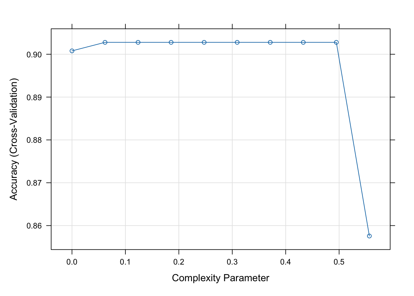

tree_model2$bestTune

         cp
9 0.4947791

# Predict using new the model
predictions <- predict(tree_model2, validation_data_DT)

# Ensure predictions are factors with the same levels as the actual data
predictions <- factor(predictions, levels = levels(validation_data_DT$Economy_status_Developed))

# Compute confusion matrix
confusion_Matrix_dt <- confusionMatrix(predictions, validation_data_DT$Economy_status_Developed)
print(confusion_Matrix_dt)

Confusion Matrix and Statistics

          Reference
Prediction   0   1
         0 654  59
         1  27 118
                                         
               Accuracy : 0.8998         
                 95% CI : (0.8777, 0.919)
    No Information Rate : 0.7937         
    P-Value [Acc > NIR] : < 2.2e-16      
                                         
                  Kappa : 0.672          
                                         
 Mcnemar's Test P-Value : 0.0008293      
                                         
            Sensitivity : 0.9604         
            Specificity : 0.6667         
         Pos Pred Value : 0.9173         
         Neg Pred Value : 0.8138         
             Prevalence : 0.7937         
         Detection Rate : 0.7622         
   Detection Prevalence : 0.8310         
      Balanced Accuracy : 0.8135         
                                         
       'Positive' Class : 0

Sensitivity: 96.04%

Specificity: 66.67%

Overall Accuracy: 89.98%

# Visualize the first model
print(rpart.plot(tree_model))

$obj
n= 2006 

node), split, n, loss, yval, (yprob)
      * denotes terminal node

1) root 2006 415 0 (0.79312064 0.20687936)  
  2) Life_expectancy< 77.45 1629 111 0 (0.93186004 0.06813996) *
  3) Life_expectancy>=77.45 377  73 1 (0.19363395 0.80636605) *

$snipped.nodes
NULL

$xlim
[1] -0.65  1.65

$ylim
[1] -0.6  1.6

$x
[1] 0.50000000 0.03831241 0.96168759

$y
[1] 0.91704414 0.05269236 0.05269236

$branch.x
  [,1]       [,2]      [,3]
x  0.5 0.03831241 0.9616876
    NA 0.03831241 0.9616876
    NA 0.50000000 0.5000000

$branch.y
      [,1]      [,2]      [,3]
y 1.112783 0.2484309 0.2484309
        NA 0.7013644 0.7013644
        NA 0.7013644 0.7013644

$labs
[1] "0\n0.21\n100%" "0\n0.07\n81%"  "1\n0.81\n19%" 

$cex
[1] 1

$boxes
$boxes$x1
[1]  0.39365767 -0.05058696  0.87278822

$boxes$y1
[1]  0.78292839 -0.08142339 -0.08142339

$boxes$x2
[1] 0.6063423 0.1272118 1.0505870

$boxes$y2
[1] 1.1127827 0.2484309 0.2484309


$split.labs
[1] ""

$split.cex
[1] 1 1 1

$split.box
$split.box$x1
[1] 0.1591808        NA        NA

$split.box$y1
[1] 0.6397416        NA        NA

$split.box$x2
[1] 0.8408192        NA        NA

$split.box$y2
[1] 0.7629872        NA        NA

# Visualize the tuned model
print(rpart.plot(tree_model2$finalModel))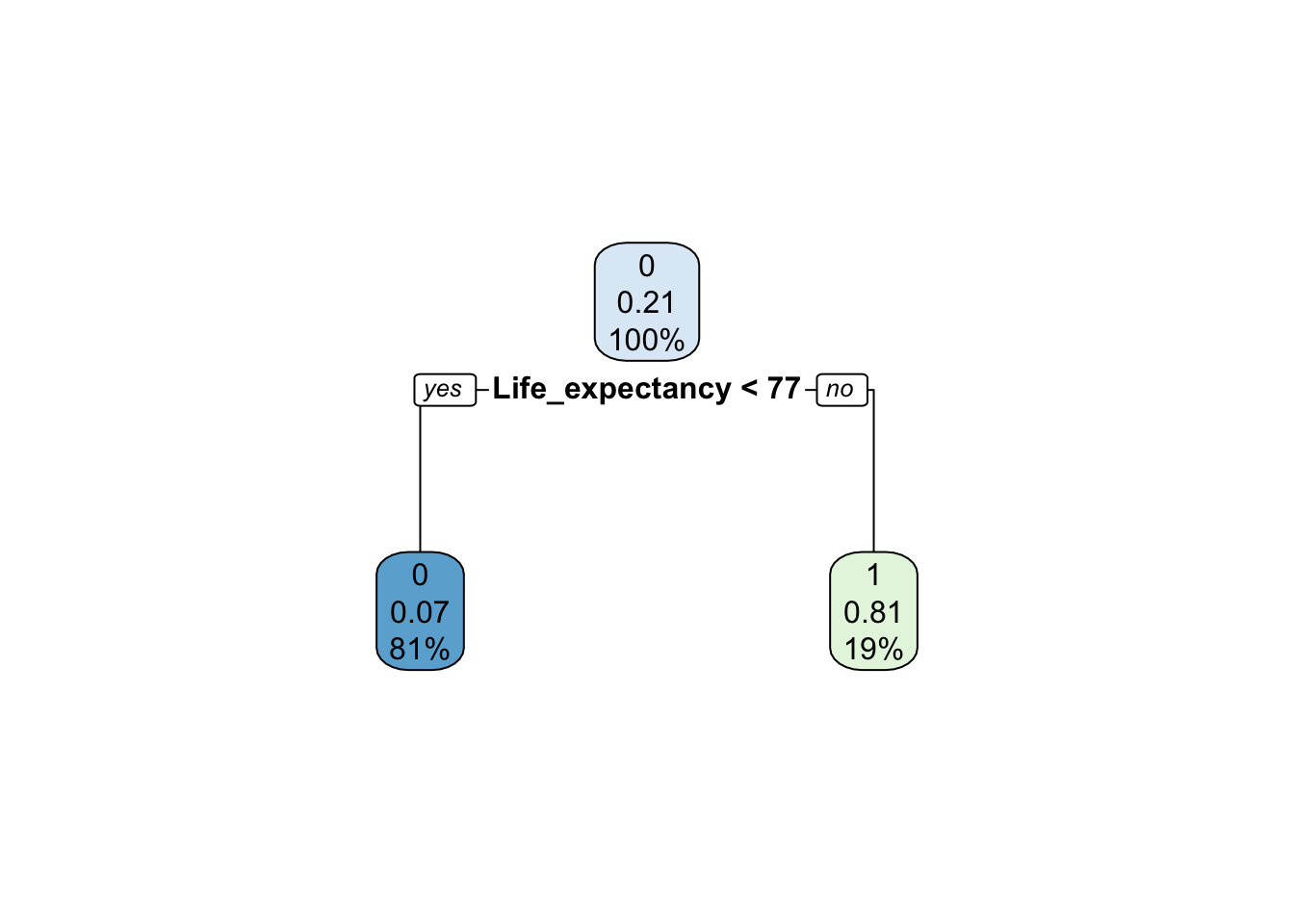

$obj
n= 2006 

node), split, n, loss, yval, (yprob)
      * denotes terminal node

1) root 2006 415 0 (0.79312064 0.20687936)  
  2) Life_expectancy< 77.45 1629 111 0 (0.93186004 0.06813996) *
  3) Life_expectancy>=77.45 377  73 1 (0.19363395 0.80636605) *

$snipped.nodes
NULL

$xlim
[1] -0.65  1.65

$ylim
[1] -0.6  1.6

$x
[1] 0.50000000 0.03831241 0.96168759

$y
[1] 0.91704414 0.05269236 0.05269236

$branch.x
  [,1]       [,2]      [,3]
x  0.5 0.03831241 0.9616876
    NA 0.03831241 0.9616876
    NA 0.50000000 0.5000000

$branch.y
      [,1]      [,2]      [,3]
y 1.112783 0.2484309 0.2484309
        NA 0.7013644 0.7013644
        NA 0.7013644 0.7013644

$labs
[1] "0\n0.21\n100%" "0\n0.07\n81%"  "1\n0.81\n19%" 

$cex
[1] 1

$boxes
$boxes$x1
[1]  0.39365767 -0.05058696  0.87278822

$boxes$y1
[1]  0.78292839 -0.08142339 -0.08142339

$boxes$x2
[1] 0.6063423 0.1272118 1.0505870

$boxes$y2
[1] 1.1127827 0.2484309 0.2484309


$split.labs
[1] ""

$split.cex
[1] 1 1 1

$split.box
$split.box$x1
[1] 0.1591808        NA        NA

$split.box$y1
[1] 0.6397416        NA        NA

$split.box$x2
[1] 0.8408192        NA        NA

$split.box$y2
[1] 0.7629872        NA        NA

Pruning the tree has made no change in the model. Which, thinking about it makes sense. There isn’t anything to prune.

Make the ROC Curve:

prob_predictions <- predict(tree_model2, validation_data_DT, type = "prob")


roc_curve <- roc(validation_data_DT$Economy_status_Developed, prob_predictions[,2])

Setting levels: control = 0, case = 1

Setting direction: controls < cases

plot(roc_curve, main="ROC Curve" , print.auc = TRUE, print.thres ="best")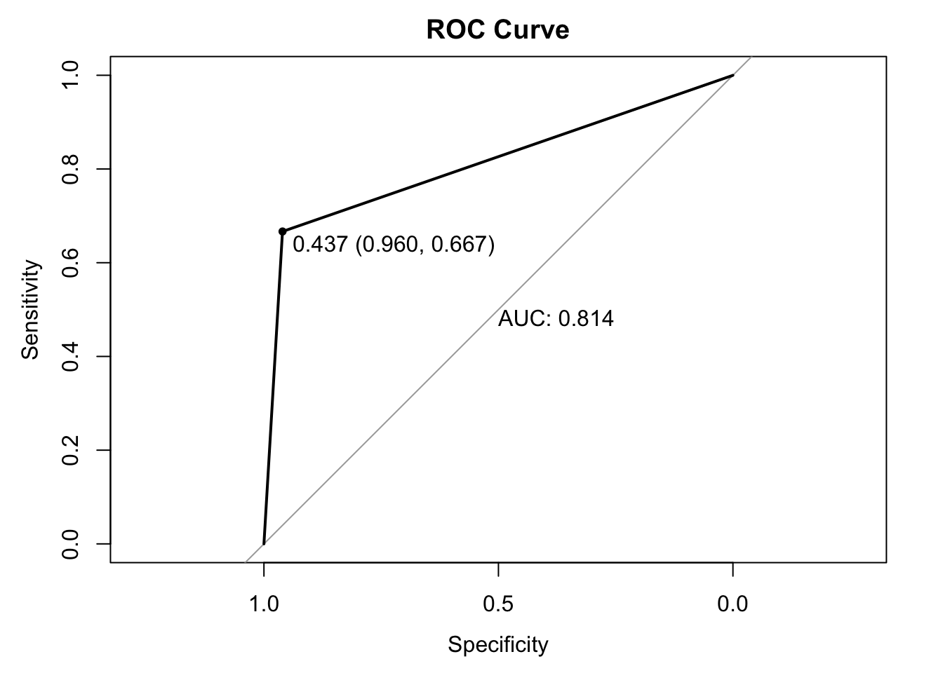

5.7.4 Comparing the Models

	Logistic	Tree	XGBoost
Specificity	83.05%	66.67%	67.59%
Sensitivity	91.5%	96.04%	96.34%
Overall	89.76%	89.98%	90.90%

For Specificity (Minimize False Positives) the logistic model is the winner, For Sensitivity (Minimize False Negatives) both the decision tree and the XGBoost are comparable.

However none of these models were made with either in mind, and these values could be fine tuned via the ROC Curves provided with each to specialize in either. However our data set doesn’t include any costs for False Positives or negatives, and as such it is difficult to determine a “Best.”

5.8 Deep Analysis

Across almost all of our plots, Africa is the lowest when it comes to life expectancy and the highest when it comes to mortality. Why is that? We will be looking at Africa in depth in order to possibly explain this.

ggplot(df, aes(x = Under_five_deaths, y = Region)) +
  geom_point() +              
  labs(title = "Region vs Under Five Deaths")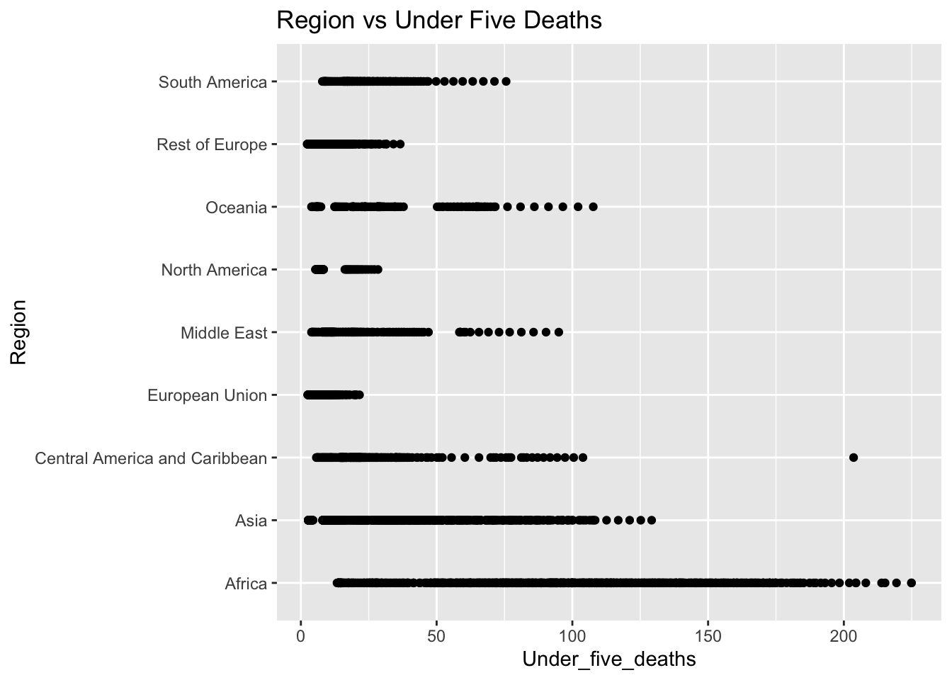

ggplot(df, aes(x = Adult_mortality, y = Region)) +
  geom_point() +              
  labs(title = "Region vs Adult Mortality")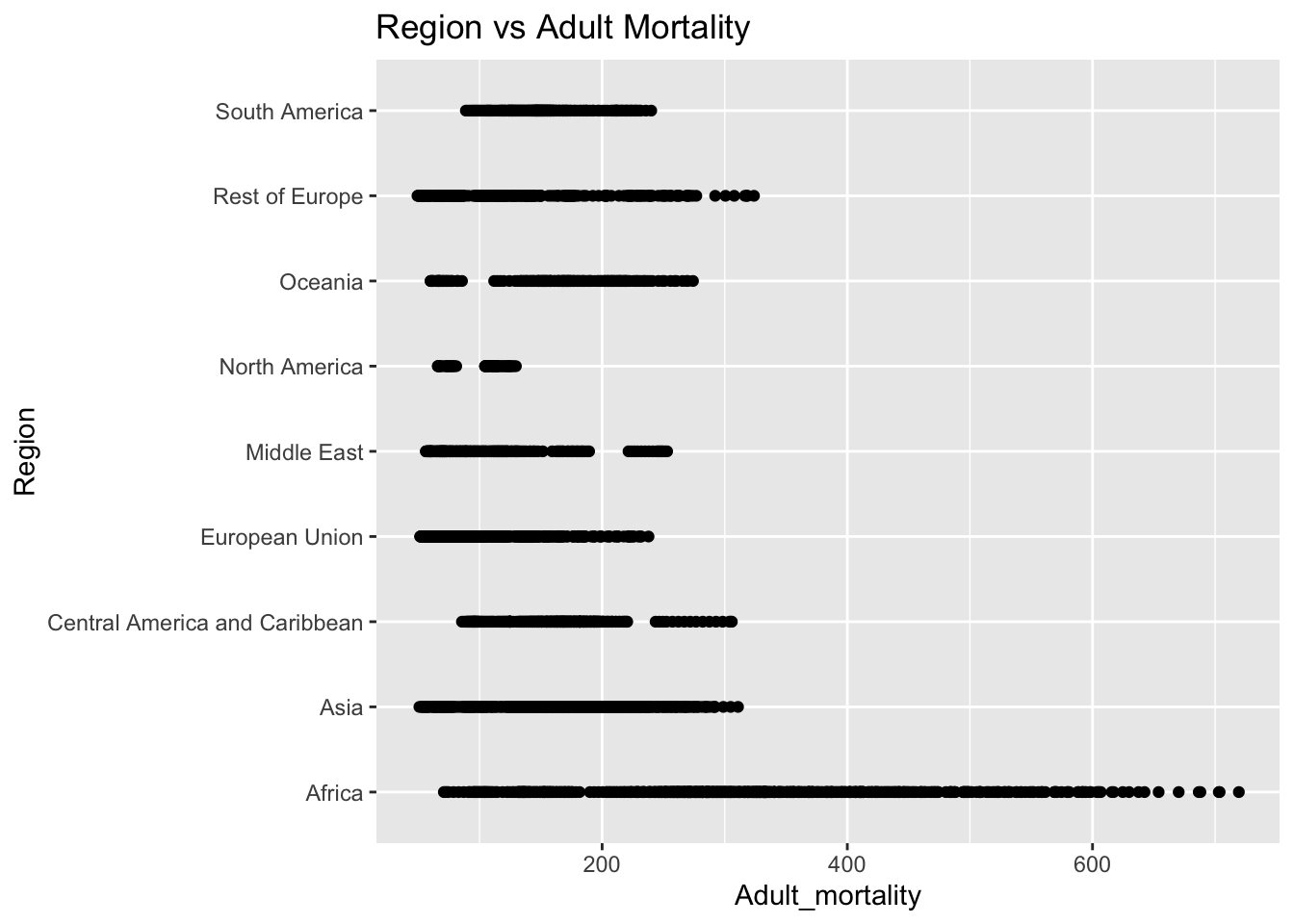

Combining under five deaths and Adult Mortality into one general Mortality variable, note that this will have a gap between 5 and 15, and anyone above 60 will be excluded in this metric.

df$Mortality <- df$Under_five_deaths + df$Adult_mortality

ggplot(df, aes(x = Mortality, y = Region)) +
  geom_point() +              
  labs(title = "Region vs Mortality")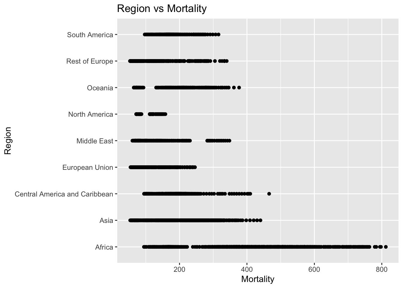

Next we will break down Africa into the countries within it for further analysis, and examine each variable in our data set this way to look for possible explanations.

filtered_df <- df %>%
  filter(Region == "Africa")
ggplot(filtered_df, aes(x = Mortality, y = Country)) +
  geom_point() +              
  labs(title = "Region vs Mortality")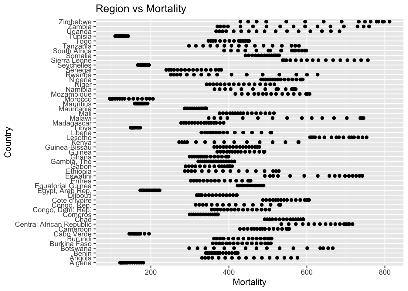

ggplot(filtered_df, aes(x = BMI, y = Country)) +
  geom_point() +              
  labs(title = "African Country vs BMI")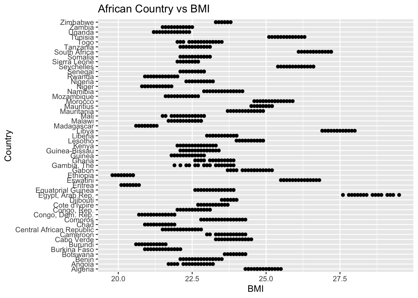

ggplot(filtered_df, aes(x = Alcohol_consumption, y = Country)) +
  geom_point() +              
  labs(title = "African Country vs Alcohol")

ggplot(filtered_df, aes(x = Hepatitis_B, y = Country)) +
  geom_point() +              
  labs(title = "African Country vs Hepatitis")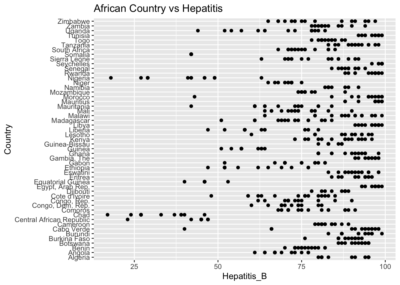

ggplot(filtered_df, aes(x = Measles, y = Country)) +
  geom_point() +              
  labs(title = "African Country vs Measles")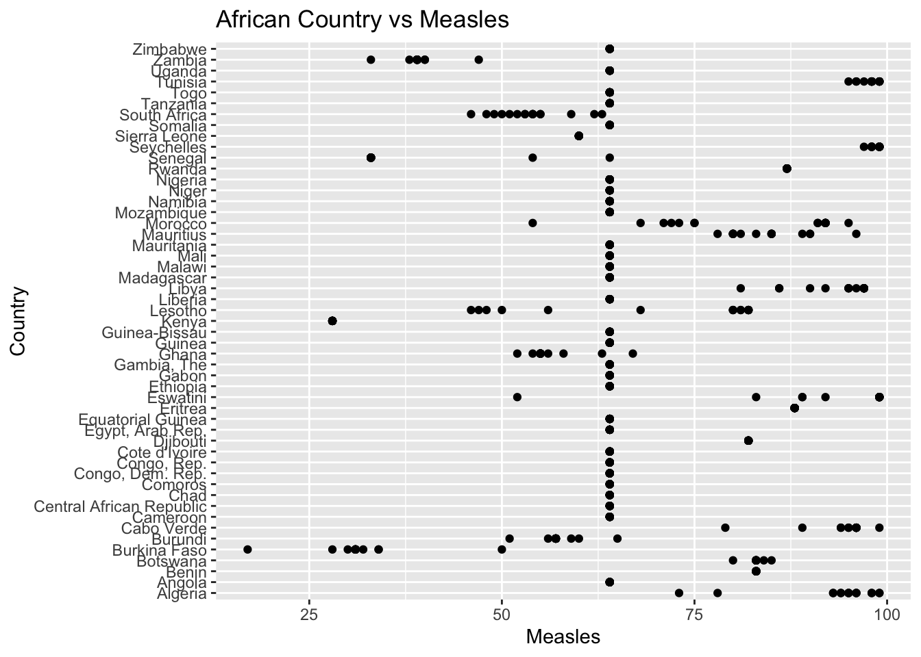

ggplot(filtered_df, aes(x = Polio, y = Country)) +
  geom_point() +              
  labs(title = "African Country vs Polio")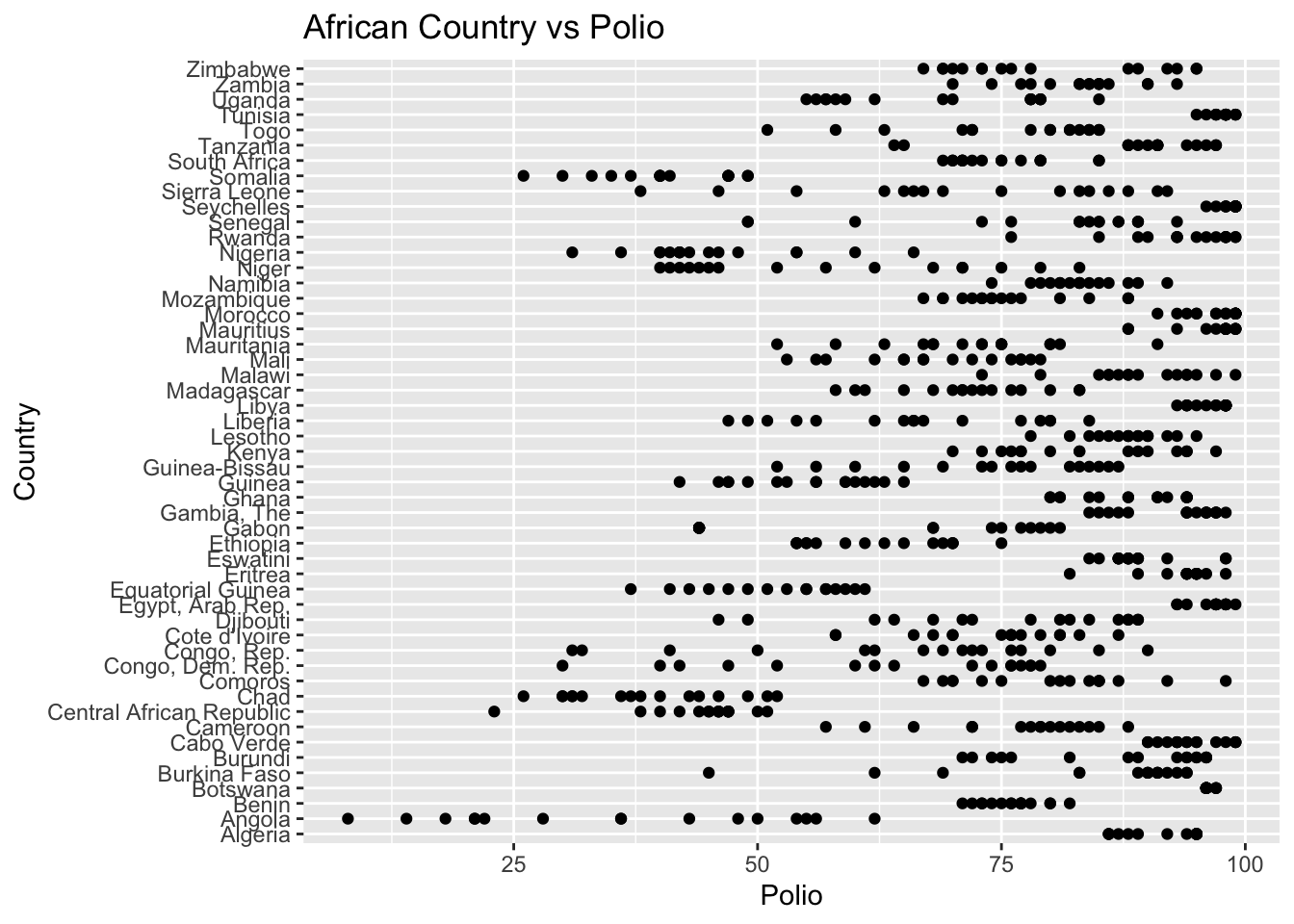

ggplot(filtered_df, aes(x = Diphtheria, y = Country)) +
  geom_point() +              
  labs(title = "African Country vs Diphtheria")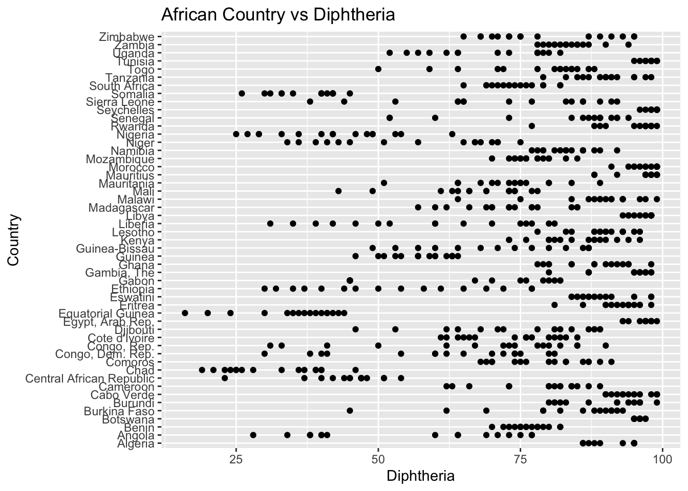

ggplot(filtered_df, aes(x = Incidents_HIV, y = Country)) +
  geom_point() +              
  labs(title = "African Country vs HIV")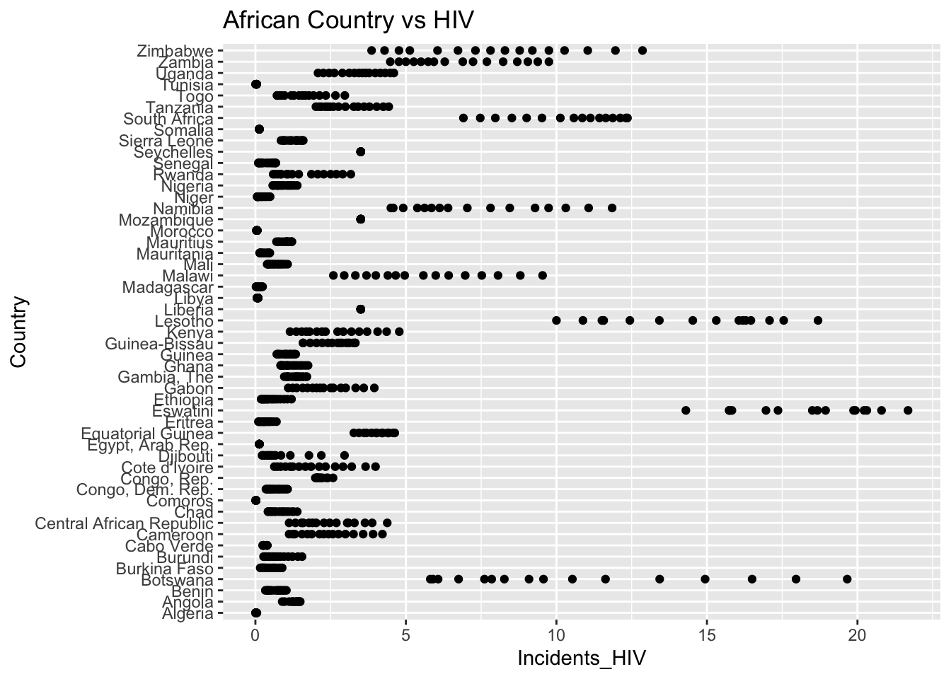

ggplot(filtered_df, aes(x = GDP_per_capita, y = Country)) +
  geom_point() +              
  labs(title = "African Country vs GDP")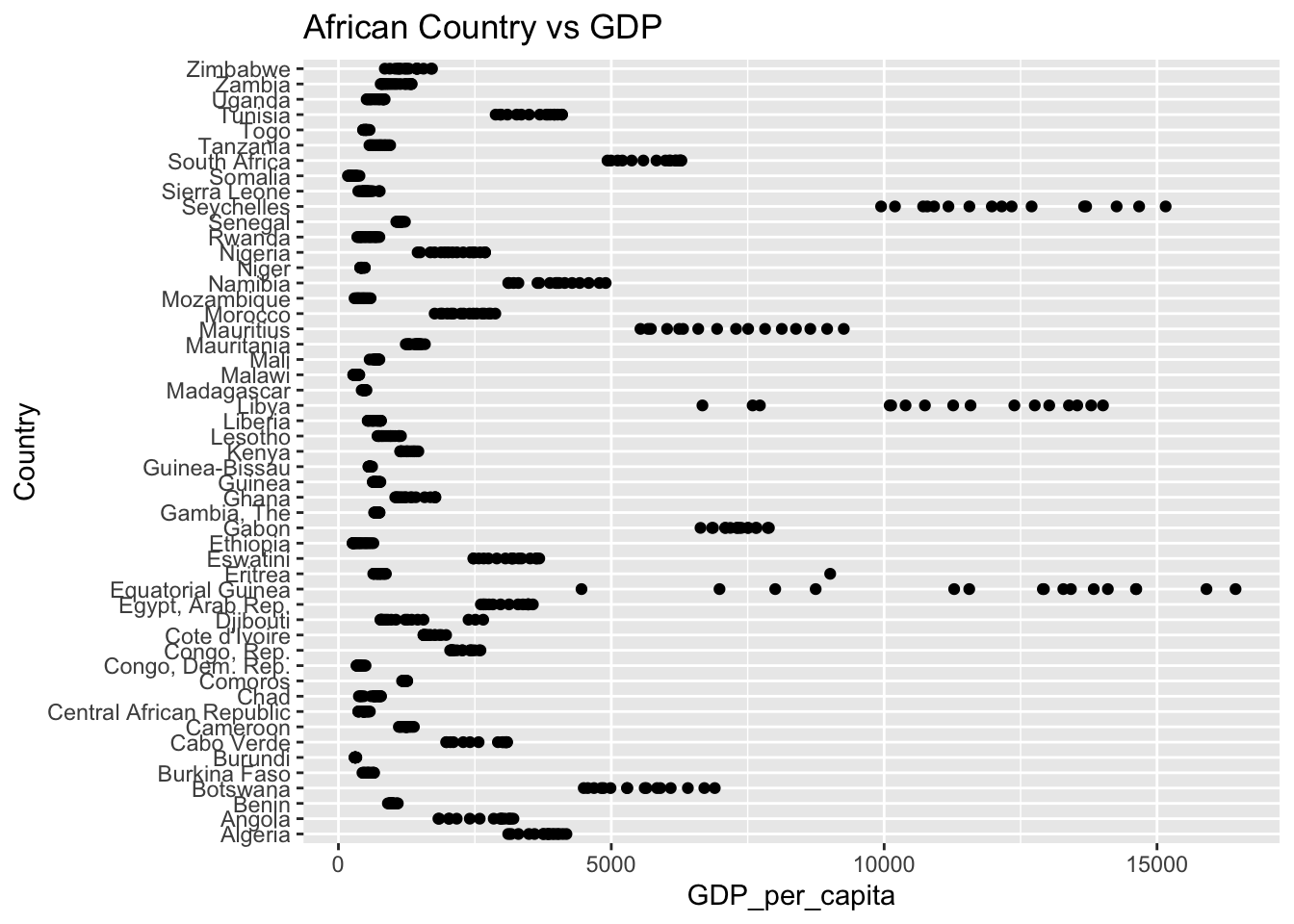

ggplot(filtered_df, aes(x = Population_mln, y = Country)) +
  geom_point() +              
  labs(title = "African Country vs Population")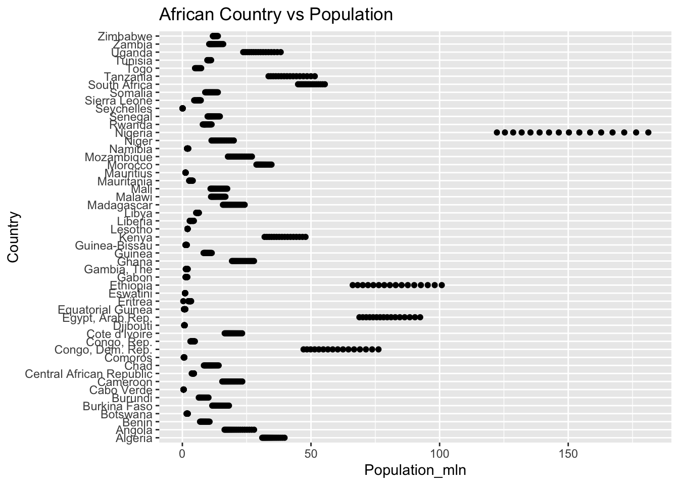

ggplot(filtered_df, aes(x = Thinness_ten_nineteen_years, y = Country)) +
  geom_point() +              
  labs(title = "African Country vs Thinness")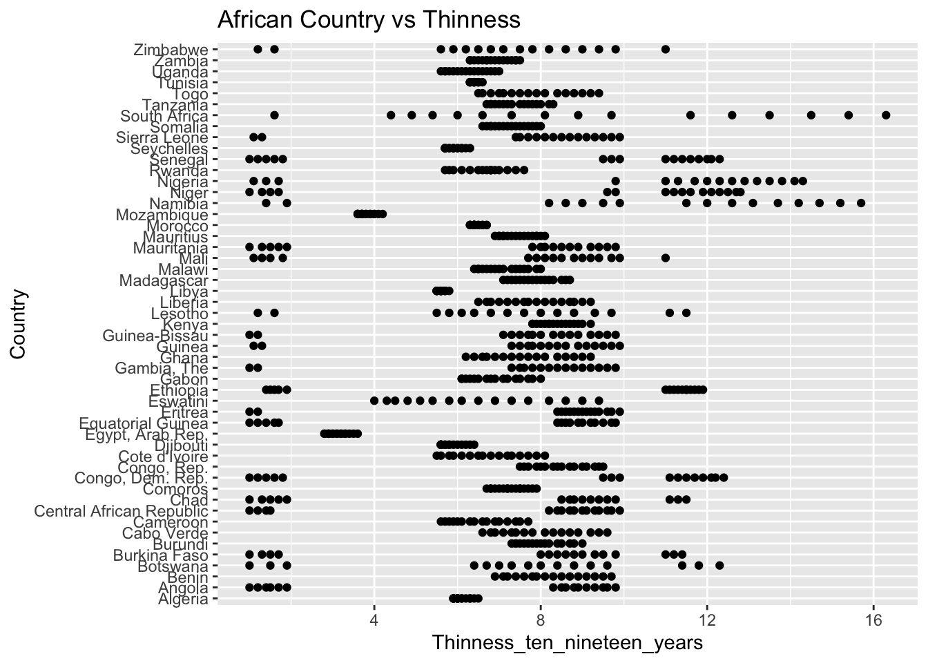

ggplot(filtered_df, aes(x = Schooling, y = Country)) +
  geom_point() +              
  labs(title = "African Country vs Schooling")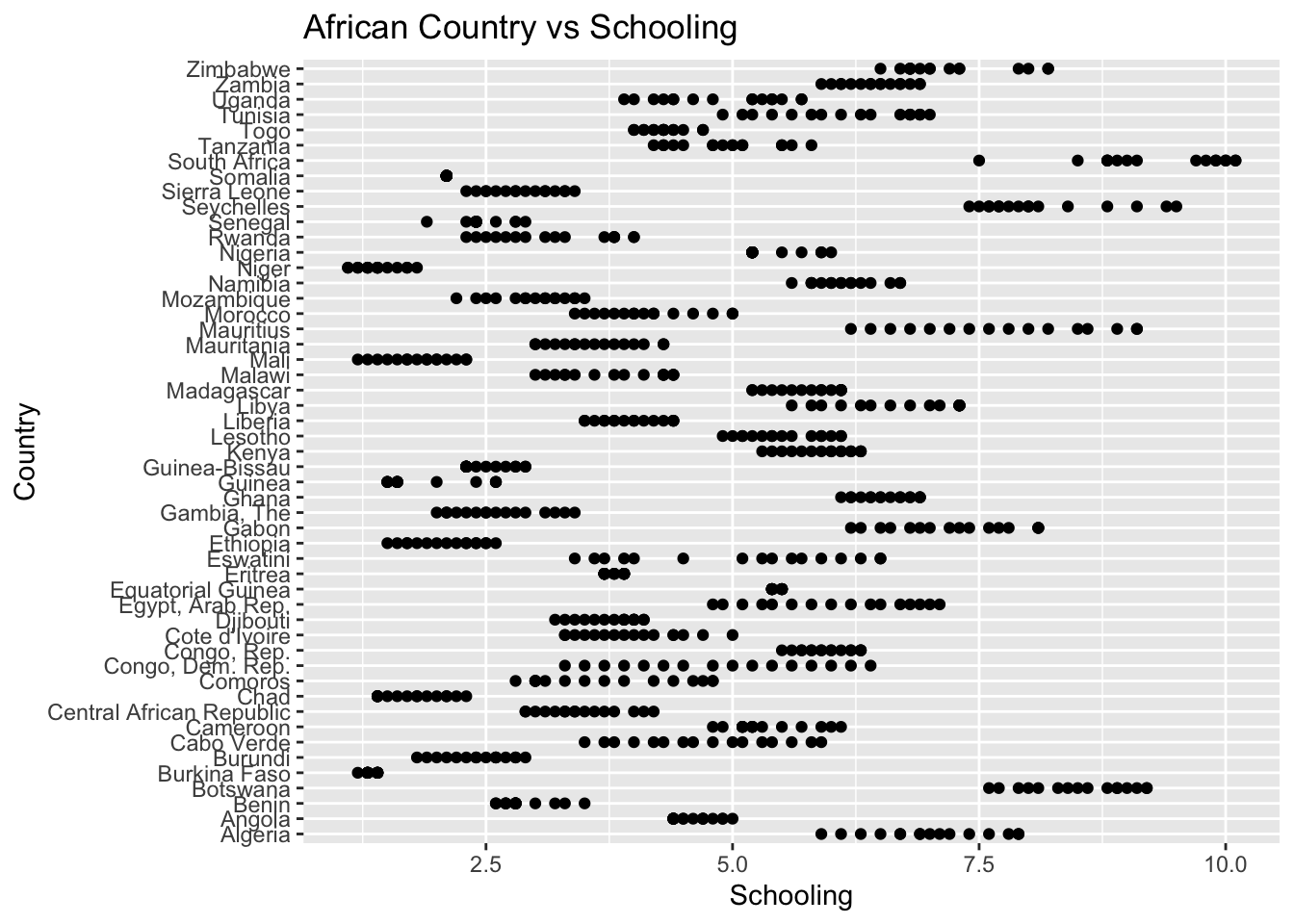

Not every African nation is low in life expectancy, Why is that? We will take out the two highest, and two lowest countries in Africa and examine them fully, taking the average of the variables within our data over the 15 years present within the data set.

Country	Mortality	BMI	Alcohol	Hepatitis B	Measles	Polio	Diphtheria	HIV
Tunisia	120	25.69	1.29	96.75%	97.81%	97.69%	97.69%	0.03
Algeria	150	24.87	0.40	88.31%	93.25%	91.75%	91.88%	0.02
Zimbabwe	600	23.54	2.90	79.56%	64.00%	79.60%	79.10%	8.0
Lesotho	690	24.49	2.62	86.63%	70.44%	87.75%	89.56%	14.35
United States	116	28.27	8.60	91.5%	86.00%	92.25%	95.13%	0.13

Country	GDP	Population
Tunisia	3585.63	10.39
Algeria	3745.13	34.82
Zimbabwe	1290.6	12.5
Lesotho	926.69	2.01
United States	52662.94	302.10

filtered_us <- df %>%
  filter(Country == "United States")
ggplot(filtered_us, aes(x = Mortality, y = Country)) +
  geom_point() +              
  labs(title = "United States vs Mortality")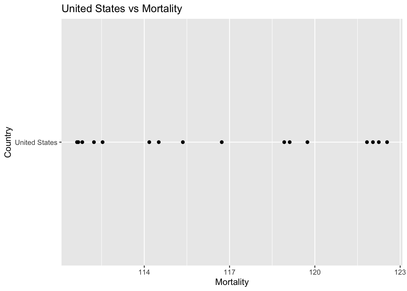

ggplot(filtered_us, aes(x = BMI, y = Country)) +
  geom_point() +              
  labs(title = "United States vs BMI")

ggplot(filtered_us, aes(x = Alcohol_consumption, y = Country)) +
  geom_point() +              
  labs(title = "United States vs Alcohol")

ggplot(filtered_us, aes(x = Hepatitis_B, y = Country)) +
  geom_point() +              
  labs(title = "United States vs Hepatitis")

ggplot(filtered_us, aes(x = Measles, y = Country)) +
  geom_point() +              
  labs(title = "United States vs Measles")

ggplot(filtered_us, aes(x = Polio, y = Country)) +
  geom_point() +              
  labs(title = "United States vs Polio")

ggplot(filtered_us, aes(x = Diphtheria, y = Country)) +
  geom_point() +              
  labs(title = "United States vs Diphtheria")

ggplot(filtered_us, aes(x = Incidents_HIV, y = Country)) +
  geom_point() +              
  labs(title = "United States vs HIV")

ggplot(filtered_us, aes(x = GDP_per_capita, y = Country)) +
  geom_point() +              
  labs(title = "United States vs GDP")

ggplot(filtered_us, aes(x = Population_mln, y = Country)) +
  geom_point() +              
  labs(title = "United States vs Population")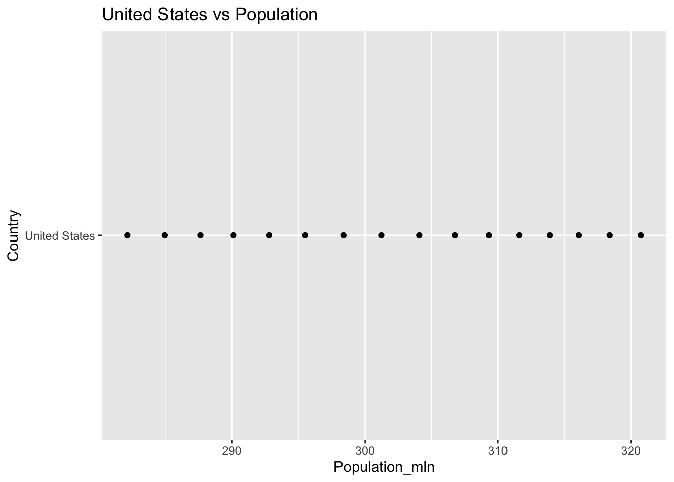

ggplot(filtered_us, aes(x = Thinness_ten_nineteen_years, y = Country)) +
  geom_point() +              
  labs(title = "United States vs Thinness")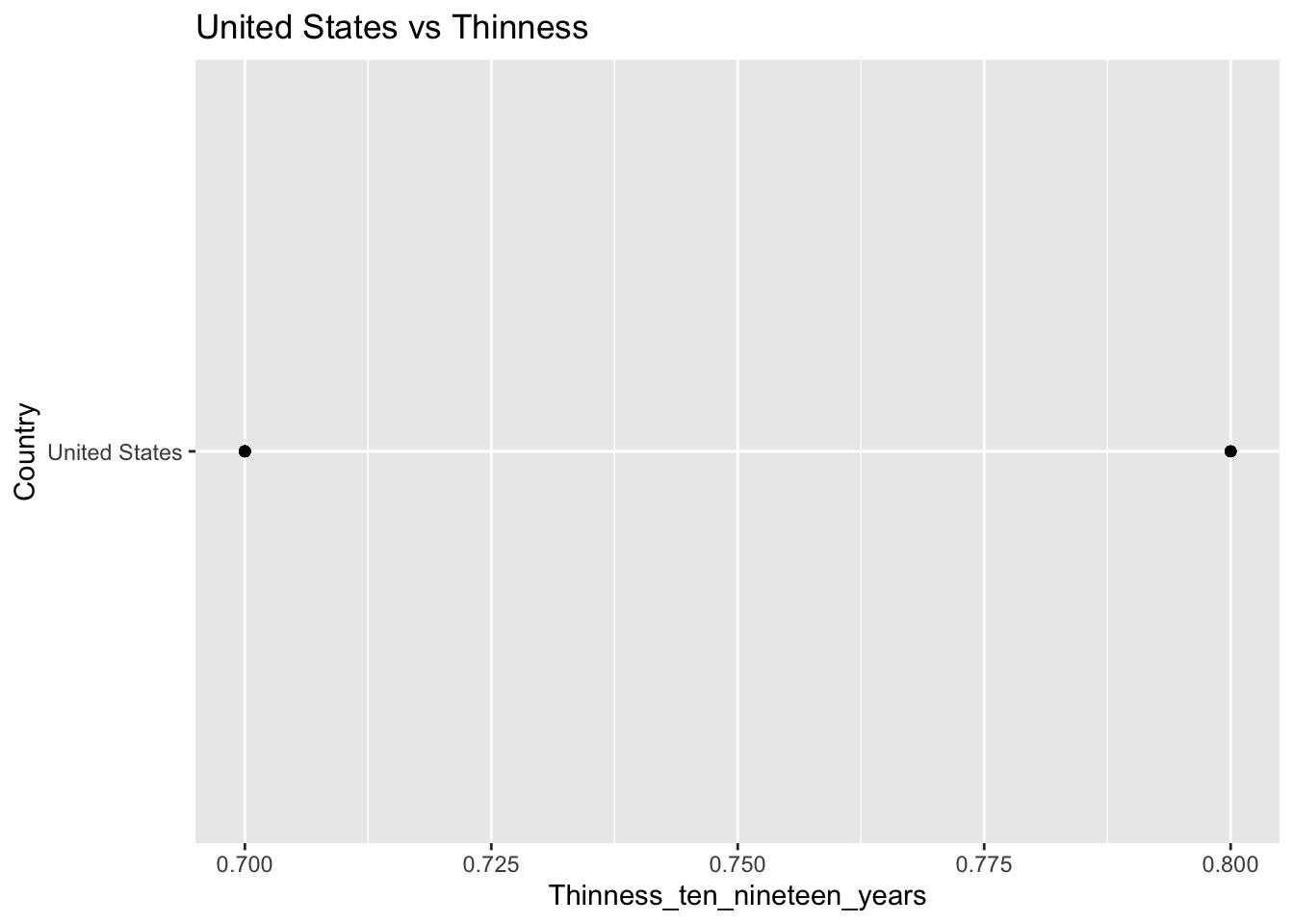

ggplot(filtered_us, aes(x = Schooling, y = Country)) +
  geom_point() +              
  labs(title = "United States vs Schooling")

5.8.1 Deep Analysis Conclusion

Tunisia and Algeria have lower mortality rates compared to Zimbabwe and Lesotho due to higher vaccination rates, higher GDP, and lower incidents of HIV.

Table of Contents

Introduction

1.1 Data Understanding

1.2 Data Source

1.3 Initial Questions

Data Loading & Understanding

2.1 Importing Libraries

2.2 Loading and Understanding the Data

2.3 Categorizing the Datasets Attributes

Data Cleaning

3.1 Handling Null Values

3.1.1 Treating Null Values

3.1.2 Decision for Treating Null Values

3.1.3 Approach

3.2 Handling Outliers

3.2.1 Explanation & Insights:

3.2.2 Treating Outliers

3.2.3 Decision for Treating Outliers

Data Analysis

4.1 Plots

4.2 Variance Analysis

4.3 Covariance Analysis

Models

5.1 Multiple Regression of Life Expectancy

5.1.1 Splitting the Data

5.1.2 Making the First Model

5.1.3 Pruning the Model

5.2 Neural Network of Life Expectancy

5.3 SVR model for Life Expectancy

5.3.1 Conclusion of SVR Model

5.4 Random Forest

5.5 Which Variables Most Influence Life Expectancy

5.6 Comparing the Models

5.7 Predict Countries Economic Status from Life Expectancy

5.7.1 Logistic Regression Model

5.7.2 XG Boost Model

5.7.3 Decision Tree

5.7.4 Comparing the Models

5.8 Deep Analysis

5.8.1 Deep Analysis Conclusion